

Modern RF Transceivers represent more than just separated receiver and transmitter functionalities within the same box. In an operational scenario involving several transceivers, even a “perfect” receiver can demonstrate high-end performance only if the spectral purity of the transmit signals is sufficiently high. Therefore, a transceiver design must align major RF parameters and building blocks between transmit and receive paths to form a combined optimized transceiver architecture! In the following, a state-of-the-art “perfect” transceiver architecture is described. This is a full length version of the article that appeared in our Oct issue here.
When a receiver and transmitter are operated at different locations and far away from each other the only relevant receive parameter is sensitivity while the only relevant transmit parameter is output power. The closer a transmitter is to the receiver, the more significant are additional performance characteristics for both. While the receiver must increase its robustness to withstand the strong transmit signal at its front-end, the transmitter must increase its spectral purity to ensure that no spectral component from the transmit signal falls into an adjacent receive channel.
In some installations, transmit signals can be extremely strong at the receiver input, while their frequencies may also be simultaneously close to the receive channels. Overall system performance is determined by the minimum usable frequency offset between a transmit channel and a receive channel with a given decoupling between a receiver and a transmitter operating a given output power.
This so-called co-site situation directly influences the specifications, for example, the adjacent channel power ratio (ACPR) for the radio communication equipment. Within a particular frequency band and its typical applications, the operating parameters may lead to a totally different transceiver architecture when compared to different applications in other frequency bands. Consequently, a transceiver for a 5G mobile phone base station, for example, may look completely different than a mobile phone base station designed to operate in the HF, VHF or UHF Band.
While the best architecture for communication equipment in a particular frequency band may vary slightly, for simplicity we focus only on systems below 600 MHz.
DERIVATION OF KEY PARAMETERS FOR SPECIFICATIONS
The transceiver RF design is directly driven by some key parameters whose values and ranges strongly influence the required circuits and the concepts for major building blocks designed to meet system requirements. Therefore, it is highly recommended to define the worst-case system scenario with respect to RF power levels and frequency offsets and derive the key parameters from this setup.
It is reasonable to assume that such a system is built up using several transceivers of the same type that are operated either in a receive or transmit mode. This allows system performance to be enhanced by optimizing the receive and transmit paths as parts of a common transceiver RF architecture. Some building blocks will be shared between receive and transmit paths, which allows simplification of the overall architecture. Typical shareable building blocks may be analog RF filters and low-noise RF signal sources used for analog mixing or as clocks for signal processing stages.
Figure 1 is one example of a system setup. Based on the output power of the transmitter, total decoupling of the transmitter spectrum at the receiver input can be calculated (see Figure 2). This spectrum view is now the basis to derive further data for the receiver and the transmitter.

Figure 1 Co-location scenario for a transceiver.

Figure 2 Total spectrum at the receiver input.
If, for example, a desired sensitivity for the receiver without any interference from a transmitter is chosen, the corresponding noise figure (NF) for the receiver front-end can be calculated. The value of – 174 dBm/Hz represents the natural noise floor power spectral density (PSD) caused by thermal effects at room temperature (kT). The NF of the receiver is then converted into a noise floor density (NFD) as follows:
NFD = – 174 dBm/Hz + NF (in dB)(1)
This sets the reference for additional external noise generated by the transmitter, which reduces the sensitivity of the receiver by adding additional noise from outside. If the external NFD from the transmitter equals that of the receiver, then the sensitivity of the receiver is reduced by 3 dB. This is called the blocking effect, or reciprocal mixing if the transmitter is active. The use of NFD instead of NF (or levels for the desired receive signals) simplifies the so-called co-site calculation significantly. With this approach, it is not necessary to know all the details about the communication method used, not even knowledge about the bandwidth.
In an operational scenario, some performance parameters must be defined with respect to a minimum remaining sensitivity. A maximum level at the receiver front-end in the presence of a transmit signal at a minimum required frequency offset relative to the receive channel must be determined. The maximum level for the transmit signal at the receiver front-end is calculated from the transmitter output power in combination with the total decoupling (in dB) between the transmitter RF output connector and the receiver RF input connector.
SPECIFICATIONS FOR A HIGH-END TRANSCEIVER
Based on the above discussion, the most important RF requirements for a wideband transceiver are identified in Tables I and II to enable high-end system transceiver performance at a radio communication site. The RF architecture to be characterized is designed to meet these criteria.
This set of requirements demands very robust input stages to enable operation in a highly contested environment. These stages use filters and amplifiers in a cascaded configuration where some elements can be bypassed. As a result, the total receiver NF with all filters active is typically 4 to 6 dB higher than expected and is on the order of 10 dB. In situations where no strong interferers are present, some co-site filters can be bypassed and additional high gain amplifiers can be activated leading to NFs on the order of 4 dB or even less.1


WHAT ABOUT RECEIVER INTERMODULATION?
The specifications in Tables I and II do not show any values for receiver intermodulation. The reason is that the definition of receiver intermodulation capability requires a more careful analysis than that shown for transmitter noise and transmitter level and its influence on receiver parameters.
Intermodulation mechanisms are responsible for effects that create unwanted receive signals when more than one interfering signal outside the receive channel is present. The most often used scenario in this context is a situation where two strong interfering signals are present at a receiver’s front-end while no receive signal is present within the receiver’s passband.
The corresponding test setup for the measurement of a receiver’s intermodulation performance is the so-called two-tone test. Two strong equal amplitude interferer signals are generated by signal generators that are tuned to frequencies outside the receiver’s passband. The two frequencies are chosen so that the intermodulation products appear within the receiver’s passband (see Figure 3).
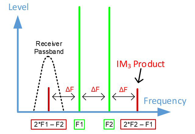
Figure 3 Two-tone receiver intermodulation test.
The two signals represented by solid green traces at frequencies F1 and F2 are the only ones applied to the receiver. The two signals represented by solid red traces are created inside the receiver passband and are processed by the receiver as external signals. The frequencies of the two red signals are 2F1-F2 and 2F2-F1, respectively and are known as intermodulation products of the third order.
With increasing levels of the two green signals, the two red signals increase significantly more due to nonlinear effects inside the receiver. When the levels of the two green signals are increased by 10 dB, for example, the internally created red signals increase, ideally, by 3 x 10 dB. In other words, the difference in level between the green and red signals is reduced by 20 dB for each 10 dB increase of the green ones. This enables a theoretical calculation of the level of the green interfering signals when the two red signals are at the same level.
This calculated level is called the intercept point third order (IP3) because with a further 1 dB increase of the green signals the red ones would then be 2 dB stronger than the green ones. The level for the IP3 is normally higher than the maximum allowed signal strength at a receiver’s front-end and should be seen as a reference value only to compare the intermodulation performance of different receivers. The IP3 value is also used to calculate the expected levels for internally generated red signals in the presence of external green interferer signals with given signal levels.
If the input IP3 (IIP3) of a single-stage amplifier measured with a two-tone signal is compared with its 1 dB compression point then the “exact” difference based on ideal mathematical models can be expected to be 9.6 dB.
In practice, the front-end of a receiver is built with a cascade of amplifiers and other stages, each with some nonlinear behavior. The combination of the individual characteristics of all components is responsible for an overall behavior that may differ from those of the single stages. For example, the overall 1 dB compression point of a receiver front-end may be the result of two amplifiers being compressed by 0.5 dB each, or some other combination.2
As a rule of thumb, the IP3 of a receiver, in practice, is typically 15 dB above a receiver’s 1 dB compression point, which is typically where another nonlinear effect called cross-modulation begins. Cross-modulation is a critical effect in systems where communication waveforms with amplitude changes or amplitude modulation are used. This is the case, for example, in systems used for air traffic control because the communication waveform used is a double sideband (DSB) amplitude modulation (AM) signal. The definition of the degree of cross-modulation is unfortunately not standardized and cannot be compared between different applications.
Cross-modulation occurs when a strong interferer drives the front-end into saturation. If an amplifier is saturated, its gain is reduced and any other low-level signal passing through the amplifier at the same time also sees some reduction of gain. As a result, the low-level signal is inverse-modulated by those parts of the interferer’s envelope that saturate the front-end (see Terms and Definitions)
An air traffic controller operating on a voice channel cross-modulated by another communication channel will not be able to communicate with pilots. Even a very high receive level will not help in this situation. The maximum operational limit of a receiver system is given by its cross-modulation threshold and not by any other parameters. If interferers are kept below the cross-modulation threshold, a receive system is basically operating within a linear area. Below this limit, reception quality is determined by key parameters of the receiver and those transmitters acting as interferers.
WHAT RECEIVER INTERMODULATION PERFORMANCE IS REQUIRED?
The relevant collocation scenario, which is the basis for the calculation of receiver parameters, is shown in Figure 1. This scenario is sufficient if only one transmitter signal acting as an interferer is present. If it is assumed that all stations involved are transceivers, then three stations are needed in total if a two-tone intermodulation calculation is done. The most important parameter for the derivation of receiver data from given transmitter data is an assumed antenna decoupling of 25 dB between the stations, which is a reasonable value for amateur radio contests and field days.