Figure 4 shows three transceiver stations, where two are transmitting while the third is receiving. The two transmitters operate at frequencies F1 and F2. The colors for the RF signals correspond to those used in Figure 3, but the sources and mechanisms for why these signals are present are different. Both transmitter signals with a power of 150 Watts (+ 52 dBm) each appear at a level of +27 dBm at the receiver’s input, which is consistent with the values in Table I.

The transmit signal of Transmitter 1 also appears with a level of +27 dBm at the antenna of Transmitter 2 because the antenna decoupling of 25 dB is valid for any combination of the antennas.

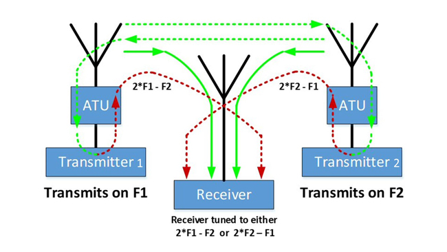
Figure 4 Two-tone interferer scenario.

This means that each transmitter is exposed to an interfering signal that is backward-radiated into its antenna. Based on a mechanism called “backward intermodulation” this transmitter creates a spurious signal that is then reradiated (see Figure 5).

The transmitter, which transmits on frequency F1 is exposed to a backward signal F2 radiated from Transmitter 2. As a rule of thumb, a modern transistor creates a new signal based on backward intermodulation effects which can be expected to be 30 dB lower than the level of the backward applied signal.

Within installations using antenna tuning units, the backward applied signal is attenuated by the selectivity of the antenna tuning unit in combination with the tuned antenna. The reradiated signal is suppressed even more because both signals appear at frequency offsets from the transmitter’s own transmit frequency. Figure 5 shows the worst-case scenario without antenna tuning units when broadband antennas are used.

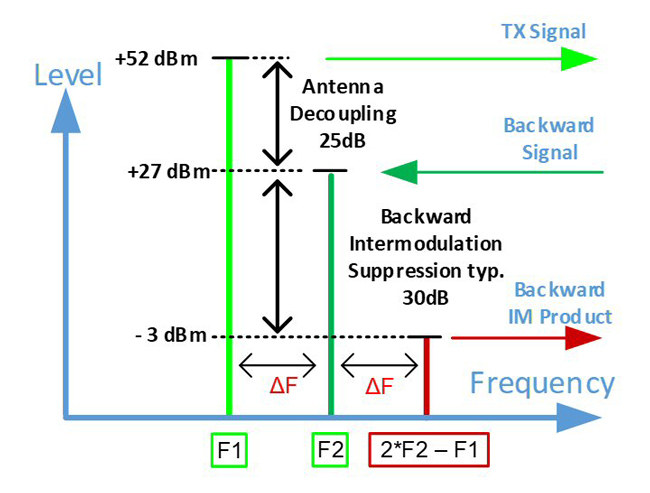
Figure 5 Spectrum at one of the transmit antennas.

At the antenna of Transmitter 2, a similar spectrum is present which is symmetrically mirrored. The transmitted spectra from both transmitter antennas are radiated to the receiver’s antenna and overlap there. As a result, the total spectrum applied to the receive antenna already contains intermodulation signals at exactly those frequencies that would be created by the receiver if no backward intermodulation signals from the transmitters were present.

Figure 6 shows the involved spectral components and their levels, which are now used to calculate a hypothetical receiver IP3. This hypothetical IP3 represents receiver performance that would lead to the same intermodulation products if only the two transmit signals were applied.

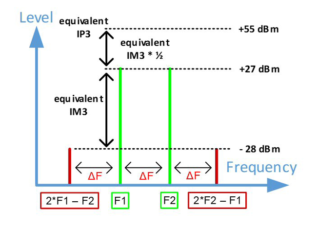
Figure 6 Spectrum at the receive antenna.

The two green lines represent the carrier levels of the two 150 Watt (+52 dBm) transmitters with an antenna decoupling of 25 dB to the receive antenna while the two red lines represent the backward intermodulation products of the two transmitters. The two backward intermodulation signals as shown in Figure 5 are also attenuated by the antenna decoupling of 25 dB and appear at a level of – 28 dBm at the receive antenna. Based on these parameters, a hypothetical receiver IP3 of +55 dBm is calculated, which is very high. These values show that it is quite unrealistic to operate a receiver at frequencies where intermodulation products may appear.²

FREQUENCY PLANNING INSTEAD OF VERY HIGH IP3

Within an operational scenario involving real transmitters, even an ideal receiver with extremely high intermodulation performance would not be able to use those frequencies for which intermodulation products may theoretically appear. The operational limits are set by the backward intermodulation performance of all involved transmitters creating signals on all potential intermodulation frequencies which are then applied to the receiver from outside.

The calculations show that all levels of intermodulation signals exceed the sensitivity threshold of a receiver by approximately 80 dB or more. For interference-free operation of those frequencies where intermodulation products may appear, both the involved transmitters and the receivers would need improvements by unrealistic orders of magnitude. This proves that the solution for interference-free operation is not a further improvement of either receiver or transmitter performance, but frequency planning.

The solution required must enable the operation of receivers and transmitters of different technologies and performance. Some large HF installations separate receiver and transmitter sites and build so-called “split site configurations” knowing that this is just a means to reduce the transmit signal levels and transmitter noise at all receiver front ends. However, this separation will not sufficiently reduce the intermodulation performance of the entire installation, because all transmitters (remaining close to each other) still create high-level backward intermodulation products at receiver locations. The question is, “How can intermodulation effects be overcome in practice?”

The only way to achieve interference-free operation is to establish a frequency planning method to avoid a situation where a receiver is tuned to a frequency where intermodulation products may theoretically appear. With large commercial stations like coastal sites or on Navy ships, frequency planning is standard using analytical tools. These tools are loaded with all frequencies that are candidates to be used and they calculate all permutations of frequencies in any combination of transmit and receive modes of all transceivers. They provide indications of potentially interfered frequencies and recommend optimized frequency channel allocations. Optimizations often prescribe just small frequency changes of some kHz for some transceivers, which puts all intermodulation products sufficiently outside a receiver’s passband.

A commercial site has all communication equipment within an installation under its control, and can, therefore, quite easily optimize the frequency plan. This situation is different for amateur radio events like field days, but frequency planning is also possible here as well if the operators are aware of the necessity.

The calculation of potentially interfered frequencies can be quite easily accomplished with a step-by-step approach if only the two strongest transmitter frequencies of all possible stations are considered. In this case, all involved frequencies are equidistant to each other for intermodulation of the third order. For intermodulation of the fifth order, the intermodulation products are double the distance from the two interferers.

In parallel and independent of that, it is recommended to operate two transmitters on two unfavorable frequencies just for test purposes to measure the intermodulation products by tuning a receiver to it. The measured levels help determine a suitable minimum required frequency shift, e.g. some kHz or more to bring the receivers into safe operation.

The calculation should be done for the operation of several amateur radio bands by different stations in parallel and for operation within the same band as well. For example, it may be that one station transmitter operates within the 10 m band and a second one operates within the 12 m band. By choosing unfavorable frequencies, in detail, intermodulation products may appear within the 15 m band. In this case, given equidistant frequencies relative to each other, a combination of one transmitter operated within the 12 m band with a second one within the 15 m band may lead to intermodulation products within the 10 m band. In this case, the introduction of a small frequency offset for one of these three stations of some kHz may be sufficient to achieve interference-free operation.

Intermodulation products within the same amateur radio band follow the same mechanism, but another significantly relevant difference in operational behavior is due to the low absolute frequency offset between the stations. In this case, it is likely that a small frequency shift will improve the intermodulation-related performance, but absolute performance will still suffer from strong transmitter noise or poor desensitization performance of the receiver. In this case, the limits as given in Tables I and II apply. After clarifying the operational context of intermodulation, no further receiver parameters need be added and the design of a transceiver architecture can begin using the parameters given in Tables I and II.

STARTING WITH THE TRANSMITTER RF CHAIN

The RF design for a transmitter can be simply seen as an RF signal generator with some amplifiers that increase the low signal level of the generator to the required high output power at the antenna.

A high-end transmitter is characterized by very low unwanted emissions outside the transmit channel. These unwanted emissions are either discrete signals or are represented by a noise floor. Discrete spurs can be caused by a variety of effects such as internal coupling of clock signals into the RF path. Other causes for discrete spurs can be nonlinearities in the transmit path, mainly within the final power amplifier. But before discrete spurs can be minimized, the basic design of the transmitter must first deliver a low noise floor, otherwise, the radiated unwanted noise may already significantly interfere with adjacent channels.

The unwanted noise floor can be separated into two different areas, which also represent two different noise-creation mechanisms (see Figure 7). The first area is close to the carrier and is normally called phase noise while the second area is far from the carrier frequency and is called broadband noise.

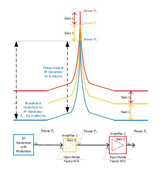
Figure 7 Total spectrum at the transmitter output.

While phase noise close to the carrier is defined by the quality of the RF generator, the broadband noise floor of the transmitter chain is mainly defined by the design of the amplifier chain behind the RF generator. Figure 7 shows where the spectrum delivered by the RF generator is simply lifted in level by two amplifiers.

For a high-end transmitter, the required broadband noise floor may be so low that even with an RF generator that produces no noise, the resulting noise floor after the amplifiers may be too high. This means that a significant improvement can only be achieved by inserting filters into the RF path. The optimization of this filter/amplifier chain must then be done by going backward from the antenna through all stages and analyzing the gain of each amplifier stage.

Figure 8 shows an improvement in the RF path by inserting two bandpass filters in front of each of the two amplifiers. The minimum broadband noise floor, which appears at the output of the transmitter, and the input to the antenna, is the noise present at the input of Amplifier 2, which is then increased by its gain.

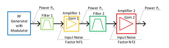
Figure 8 Improved transmitter RF path.

For a first optimization, the elements within the RF path can be seen as ideal, e.g. the filters do not have any insertion loss and the amplifiers have just an NF and a flat frequency response with a given gain. It is also assumed that a filter in front of an amplifier suppresses all broadband noise coming from previous stages completely. With this simplification, the broadband noise floor after the final amplifier is just the input noise floor represented by the amplifier NF, which is then increased by the amplifier gain.

While the output power of the RF generator inside the filters‘ passbands is increased by the amplifiers, the broadband noise floor outside the filters‘ passbands is first suppressed by the filters; then, a following amplifier just increases its input noise floor by its gain. Consequently, the output noise floor always remains quite low while the output power goes up by the total gain of the transmitter’s RF path.