Hello, fellow RF/microwave enthusiasts. My name is Abhishek Tiwari, and I am a product manager at MathWorks where I focus on products that help system architects and RF/microwave engineers design and develop wireless systems. I collaborate closely with 5G, radar and EW RF engineers, helping them use MATLAB and Simulink for building wireless systems in the most efficient way possible.

Today’s wireless systems are requiring engineers to have a comprehensive understanding of multifunctional capabilities. The evolution of RF systems from single to multifunction requires systems now to be flexible so that they can perform multiple tasks and functions that were previously performed by individual, dedicated wireless systems.

For the wireless engineer, this now means having to understand the challenges that are associated with these multiple different tasks, including phased array front ends, radar, 5G, and EW. Additionally, AI is adding to the complexity and challenges for wireless engineers as they develop these multifunctional systems.

Code & Waves is a quarterly blog that will look to examine these complexities that wireless engineers are grappling with while providing information and solutions to help in navigating this evolution, ultimately contributing to the successful development of advanced wireless technologies. This blog series will explore challenges like system complexity and crowded RF spectrum and interferences as well as solutions while also providing models, examples, and techniques to help in overcoming these daily obstacles.

In this first blog, we’ll explore modeling individual subsystems in a monopulse application. The monopulse system model is built for a transmitter and receiver antenna having four elements arranged in a rectangular array configuration of size 2-by-2. The geometry of the antenna is shown in Figure 1. The antenna pattern for transmitter and receiver at the frequency of 2 GHz is given in Figure 2 and Figure 3, respectively. The maximum value is obtained for [azimuth elevation] of [0^o 90^o] and the directivity is 14.8dBi. The same antenna is used at the receiver, but it is tilted by 180 degrees so that the two antennas face each other. The antennas are analyzed using the Antenna Toolbox’s full-wave method of moments solver which considers the mutual coupling between the antenna elements. 

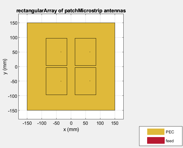Figure 1: Antenna array geometry. ©2024 The MathWorks, Inc.

Figure 2: Pattern of transmit antenna. ©2024 The MathWorks, Inc.

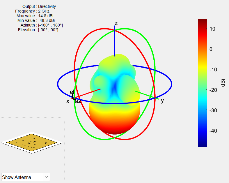Figure 3: Pattern of receive antenna. ©2024 The MathWorks, Inc.

The antenna can be designed and simulated with just three lines of code provided in Figure 4.

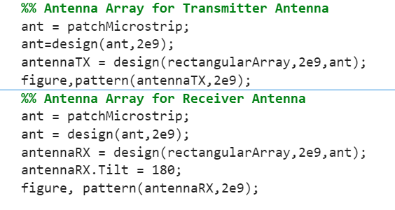
  Figure 4. Code for calculating a pattern. ©2024 The MathWorks, Inc.

Rat-race couplers are used to build the receiver analog comparator and Wilkinson power dividers are used to create the feed network of the transmit antennas. The coupler and dividers can be designed using the catalog library of RF PCB Toolbox and analyzed using the method of moments solver as shown in Figure 5.

Figure 5. Geometry of the rat-race coupler. ©2024 The MathWorks, Inc.

 The s-parameters can be saved in s3p and s4p files, respectively generated using the following code in Figure 6.

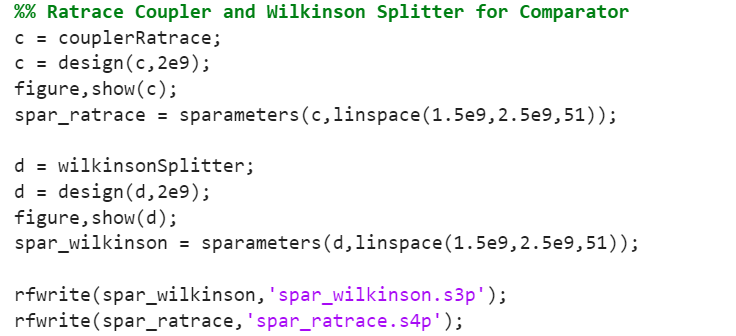
Figure 6. Code for generating s-parameters file. ©2024 The MathWorks, Inc.

Integrated System Model for Monopulse Radar

The simulation model includes the transmitter and the receiver. A 10dBm CW input signal is divided into four equal parts using Wilkinson splitter blocks and fed into the transmit array. The antenna array block is used to specify the transmitter antenna array object shown in Figure 4 and the direction of departure. Assuming far-field conditions, the receive array block specifies the array object and direction of arrival. The receiver antenna is connected to the comparator circuit, built using rat-race couplers, and the first three outputs can be used to determine the distance and relative position between transmitter and receiver. The monopulse tracking system model can be simulated with different angles of departure and arrival, and the measured power of the three outputs allow recovering the relative location between transmitter and receiver, as shown in Figure 7. The first output represents the coherent sum of the power received by the four antennas and it is proportional to the distance between transmitter and receiver. The relative phase shifts of the four signals are used to create the second and third outputs, with power proportional to the relative difference of azimuth and elevation angles between transmitter and receiver.  

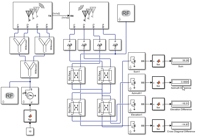Figure 7. Simulink model of the proposed system. ©2024 The MathWorks, Inc.

 To visualize the system’s behavior based on the target location, simulations were run on this model by varying the angle of arrival on the receiver array block. The angle of arrival specifies the direction from which the signal is received and mimics the behavior of the target’s location. The angle of arrival is initially specified along the boresight direction of the receiver antenna which is [0^o -90^o] and then decreased in the steps of 10 degrees to measure the power received in the sum, and azimuth-difference and elevation-difference ports. The values for different target locations are tabulated in the table below:

At boresight, the sum port gives the value of 39.2 dBm which matches with the expected result obtained by adding input power, gain of transmitter, and receiver antennas. The difference between the sum port and azimuth difference gives the null depth 20dB lower than the sum signal. A large difference between the power of the sum and difference (azimuth/elevation) signals is an indication of the radar ability to discriminate the target position. In this case, the difference needs to be improved for better performance of a monopulse system. 

The lower value of null depth observed is caused by a small phase difference between the antenna ports due to coupling effects. To compensate for this effect, phase shift blocks are connected to the output of the antenna ports. The null depth improves and is 40 dB lower than the sum signal shown in Figure 8.

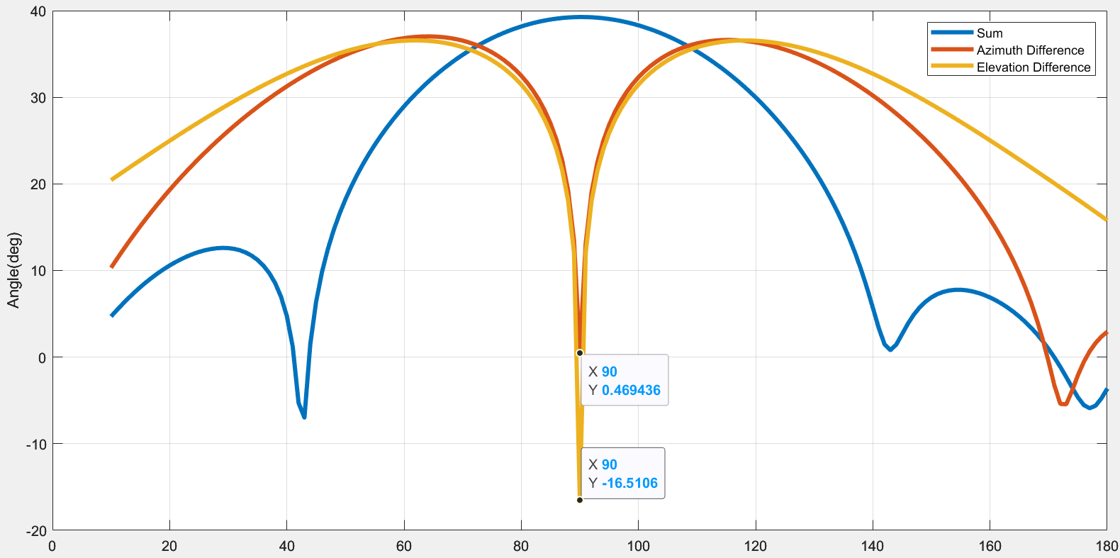
           Figure 8. Sum and difference pattern for the model. ©2024 The MathWorks, Inc.

The model can be further refined using s-parameters, calculated using a behavioral model or a method-of-moments solution. You can use Harmonic Balance and Circuit Envelope Simulation to account for non-linear effects into the simulation.

In the previous simulation and in the model shown in Figure 7, ideal blocks were used for the couplers and splitters. The Wilkinson and the rat-race coupler blocks can be replaced with s-parameters blocks using the s3p and s4p files calculated in Figure 6. The simulation results show that the null depth degrades when using realistic s-parameters computed with the method of moment electromagnetic analysis. The null is only 20 dB lower than the sum signal at the boresight as shown in Figure 9, which is what we might observe when the design is fabricated. Efficient designs of rat-race couplers which have good isolation between the ports and exact phase difference between the output ports can improve the null depth.

Figure 9. Model showing s-parameters blocks for Wilkinson and rat-race coupler. ©2024 The MathWorks, Inc.

The presented methodology shows how to improve practical designs, and simulation results prove that amplitude and phase on each branch need to be balanced perfectly to get the desired result in the monopulse system.

In this first Code & Waves blog, you saw how the monopulse system is simulated and the s-parameters of any passive structure can be used to show the monopulse tracking capability. This will reduce the time required in the design and prototyping stage and produce accurate results. Various analyses can be performed using this model by changing the antenna configurations and by using a large number of elements in the array. This model can be used for any other configuration of antenna and comparator and the system simulation can be conducted very easily.

The stage is set for the Code & Waves blog series that will guide you through the nuances, optimizations, and advancements in the field of design and testing multifunction RF systems. Stay tuned for upcoming blogs as we navigate the waves of innovation in this domain with AI, sharing valuable insights, and unlocking the potential in the world of multifunction RF systems. I hope you’ll e-mail me with your feedback and thoughts along the way.

To learn more about the topics covered in this blog and explore your own designs, see the examples below or email me at abhishet@mathworks.com.

• PCB components catalog: Learn how to create, visualize, and analyze characteristics of components like transmission lines, filters, splitters, couplers, stubs etc., used on a printed circuit board.

• Simulation of RF systems with antenna blocks: Use antenna blocks to incorporate the effect of an antenna in a RF simulation.

• Antenna and array analysis: Perform port, surface and field analysis of antenna and arrays.

• MATLAB and Simulink for RF systems: Learn how to design and evaluate multifunction RF systems like radar and wireless communications.