In this part of our blog series about voltage regulator module (VRM) characteristics, we continue to consider output impedance, Z_OUT. We’ll consider the basics of Z_OUT now and delve more deeply into academic aspects in future blog posts. As a starter for our investigation, let's see some examples of what Z_OUT looks like. 

The first step is to run a simple simulation (just as we did in part 4 of this series) and review what happens to the Z_OUT curves when the VRM turns on and off.

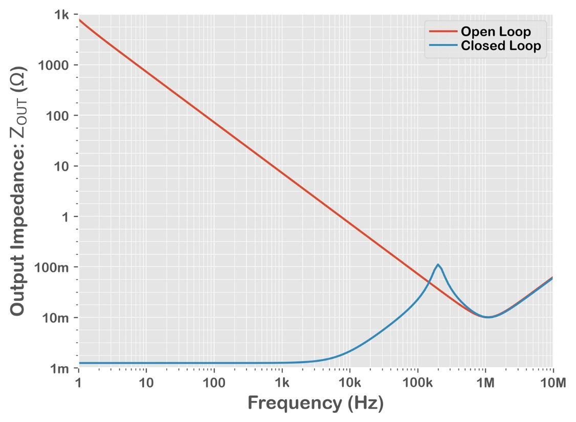
Without running a simulation, we can easily determine the Z_OUT curve shape when the VRM is off. When off, the VRM itself and the further upstream power system seen through the VRM do nothing, and our output impedance measurement setup directly measures just the output capacitor. So, our Z_{OUT(OPEN_LOOP)} figure will be mostly identical to the output capacitor impedance.

When we turn the VRM on, the regulator tries to keep its output voltage constant no matter how the output load current changes. So, the Z_{OUT(CLOSED_LOOP)} value will be lower than the Z_{OUT(OPEN_LOOP)} value.

The example simulation in Figures 1 and 2 shows the output impedance of a VRM when its regulator engine is on and off.

This simulation deck can be downloaded from the Qorvo repository at GitHub.

 

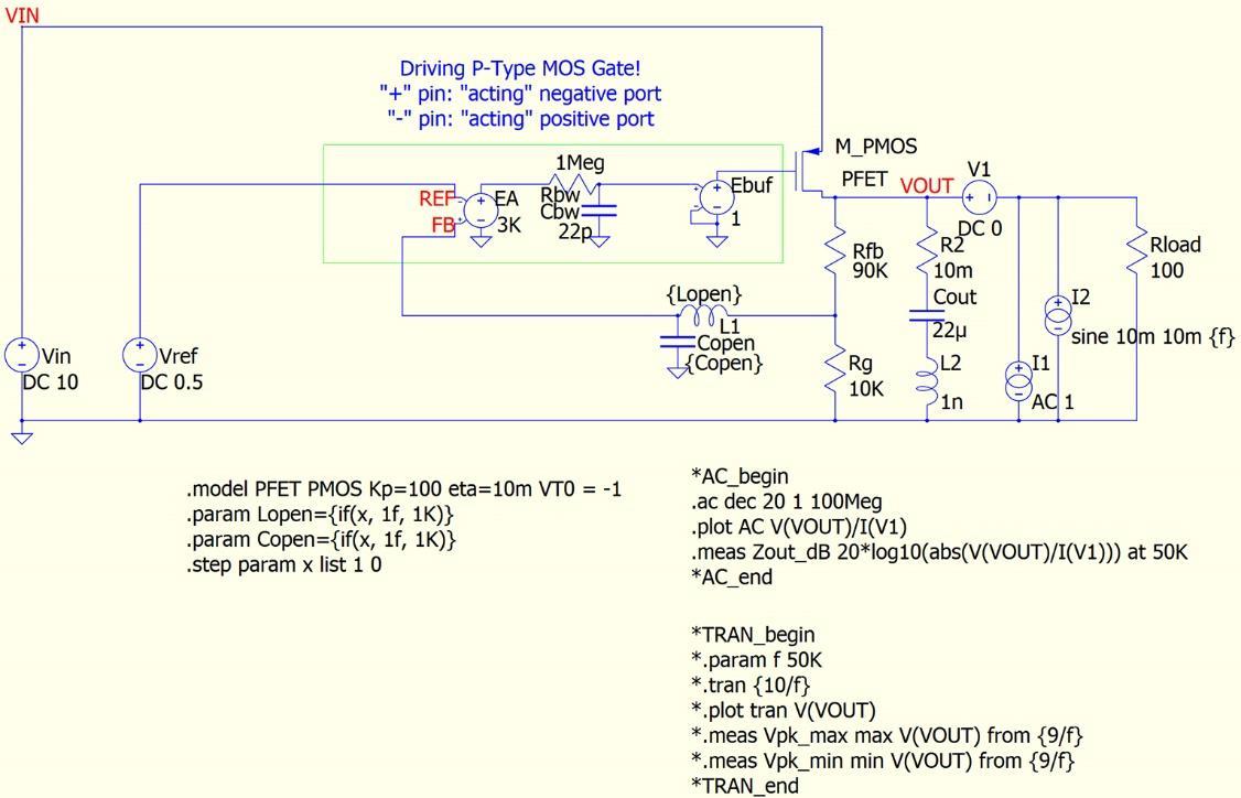
The LC pair ‘L_OPEN’ and ‘C_OPEN’ works to open/close the loop control. When closed, the gate drive signal from the error amp goes to the P-FET. When open, the gate drive signal from the error amplifier (EA) goes through this strong low-pass filter, and only the DC bias point is set by the EA. When the EA is on, we have our Z_{OUT(CLOSED_LOOP)} curve. When off, we see our Z_{OUT(OPEN_LOOP)} curve.

In this model, to make the result more realistic, we have included the ESL (equivalent series inductance) of the output capacitor along with its ESR (equivalent series resistance).

We can make the following observations and statements for Z_OUT as we did for PSRR in part 4 when we reviewed PSRR:

• When the VRM is off, we see the output capacitor impedance.
• When the VRM is on, we have the benefit of the regulator up to its control loop bandwidth. Beyond the bandwidth limit, the two Z_OUT curves are identical.

Now, we can make more observations about the output impedance: The Z_OUT curve is dominated by the output capacitor beyond the loop bandwidth (BW). In this simulation, this output capacitor block becomes just the 1 nH ESL inductor once the frequency is higher than the capacitor’s self-resonant frequency.

At higher frequencies above the VRM loop bandwidth, the Z_{OUT(CLOSED_LOOP)} value therefore shows an inductive characteristic, which is +20 dB/dec.

As frequency increases from low values, our output impedance measurement reveals the inductance of the power-conducting path(s) step by step, starting from a very low output impedance value at a low frequency with strong feedback through the VRM control loop.

Because of this ideal simulation, we can see the minimum of these two Z_OUT curves at the ESR value of 10 mΩ, as designed into the output capacitor block.

This simulation model can also be run in the time domain. The Python script in the download folder generates this plot. We compare the loop ‘on’ and ‘off’ at 50 kHz where the two output-impedance curves are close but can still illustrate their difference.

By loading the VRM with a 10 mA peak-amplitude sinusoidal current (= 20 mA peak-to-peak), this VRM model shows a small output-voltage modulation, both open and closed loop (Figure 3).

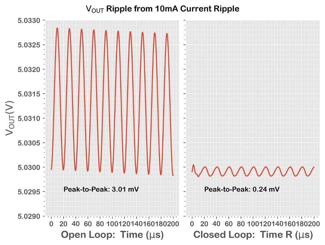
From these two time-domain waveforms, we can calculate output impedance at 50 kHz.

• Open loop:    3.01mVpp / 20mApp = 150.5mΩ
• Closed loop:  0.24mVpp / 20mApp = 12mΩ

The values match our two Z_OUT curves in Figure 2. In the next step, we measure a real-world VRM in the lab.

As a DUT (device under test), we use the VRTS1.5 ‘Voltage Regulator Test Standard’ from Picotest, the same one used in part 5 of this article series.  We also use the same VNA (Vector Network Analyzer), the Bode 100 from Omicron Lab. Figure 4 shows the arrangement.

There are various ways to measure the output impedance of VRMs, but here we will use the ‘shunt-through’ method [1]which is currently one of the most popular .

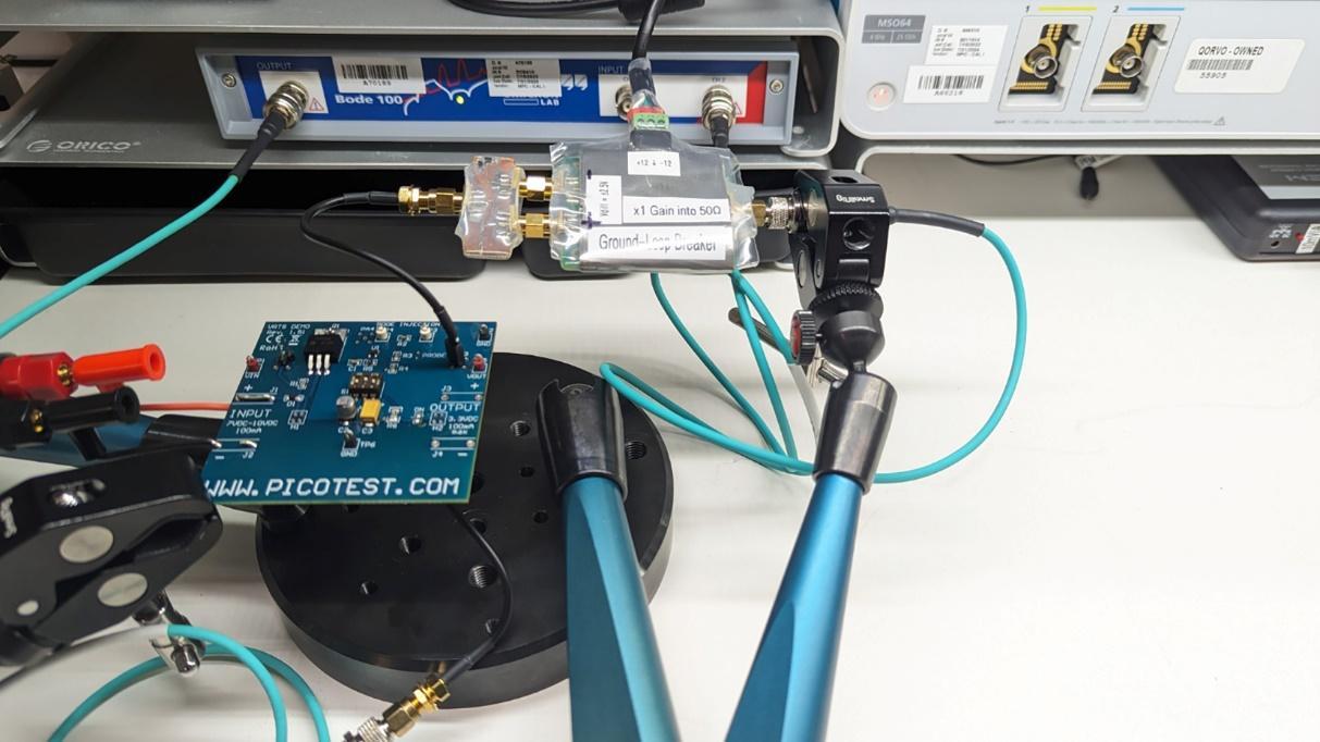
In the setup above, I’m using my own custom ground-loop breaker, but you can also find a commercial product such as the Picotest J2113A. Figure 5 shows the output impedance curves obtained.

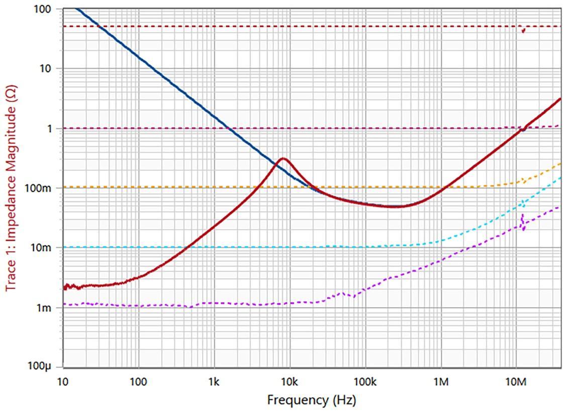
Here, the red curve represents Z_{OUT(CLOSED_LOOP)} of the VRTS1.5, and the blue curve represents Z_{OUT(OPEN_LOOP)}. To validate these measurements with known values, several reference curves are shown as dotted lines by measuring pure resistors of 1 mΩ, 10 mΩ, 100 mΩ, 1Ω and 50 Ω. 

Note that, unlike the simulation example given earlier in the blog, the measured blue curve is taken at 0V (zero volt) output of the DUT.
 
When checked, the blue curve is almost identical to the measurement of the impedance of the tantalum capacitor on the VRTS1.5 output at zero voltage bias.

Quick observations:

• The VRTS1.5 has 10 kHz control loop bandwidth, where we see a peak of Z_{OUT(CLOSED_LOOP)}
• Besides the loop bandwidth difference, the simulation result (the first half) and the actual measurement result (the second half) give us the same Z_{OUT(CLOSED_LOOP)} curve shapes.
   From low frequency to high frequency, for the closed loop curve we see:
1. VRM gain drives: flat and low impedance
2. VRM gain decreasing: +20 dB/dec increase in impedance
3. VRM gain bandwidth: positive peak
4. Above the peak, impedance follows the output capacitor value: -20 dB/dec
5. Output capacitor self-resonance: negative peak
6. Output capacitor ESL: +20 dB/dec

In this part, we have reviewed the basics of output impedance curves. From this point, we can discuss various power integrity subjects, and we will visit those topics one by one in the future parts of this series.

[1] The 2-Port Shunt-Thru Measurement and the Inherent Ground Loop (Anto Davis and Steve Sandler, Signal Integrity Journal, April 9, 2019)