
This section shows how PUL parameter functions are obtained using measured data across a given frequency range.9, 21 It shows that lumped circuit (electrically short) characteristics are used, and transmission line effects (electrically long) are ignored. This yields: L = L(f), R = R(f), C = C(f), and G = G(f).

Figure 10 Inductance in henries per meter for 1 m cables.
CFR MODELING
This section shows how CFR is calculated as a voltage transfer function using transmission line equations.9 This calculated CFR can then be compared to a measured voltage transfer function of the cable. If the comparison is a match, it implies that: 1) the PUL parameters of the cable were correctly measured and calculated and 2) the analytical expression for the CFR is correct and accurately calculated. Once it is confirmed that the analytical CFR expression is correct, G(f) can be set to zero to determine its influence on the cable CFR.
The CFR in terms of transmission line theory is equal to the output voltage divided by the input voltage, where x = ℒ at the end of the line (output) and where x = 0 at the beginning of the line (input).9, 21, 22
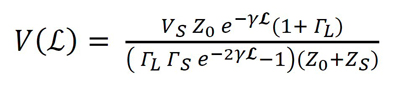
Equation (7) computes the voltage at any point on the line.9, 23
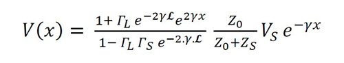
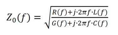
Where x is the distance along the line of length ℒ. The source voltage is VS, ZS is the source impedance and Z0 is the characteristic impedance of the cable. Z0 is a function of the PUL parameters, which in turn depends on the frequency where:24
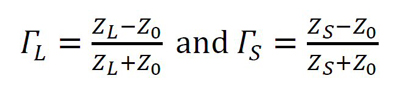
In Equation (7) there are two reflection coefficients. One for the source (ΓS) and one is for the load side (ΓL). With ZL is the load at the end of the cable. The reflection coefficients are:
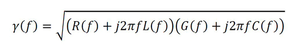
Equation (7) also contains the complex and frequency dependent propagation constant γ, where:
Equation (11) expresses the input voltage at the sending end of the transmission line by substituting x = 0 in Equation (7), which yields:

Equation (12) expresses the output voltage at the receiving end of the transmission line by substituting x = ℒ in Equation (7).
Therefore, the division of Equation (12) by Equation (11) describes the CFR as:9
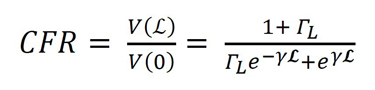
Note that in Equation (13), the source impedance and source voltage are cancelled. The CFR equation relies only on the load reflection coefficient (ΓL), the length of the cable (ℒ) and the propagation constant (γ).
CFR RESULTS
In this section, CFR’s are given for the two cables measured. These are:
• The CFR measured with a spectrum analyzer and tracking generator. This is used as a reference for the analytical equations.
• The CFR calculated by using the measured L = L(f), R = R(f), C = C(f) and G = G(f). This shows a good correlation with the measured CFR and shows that the analytical CFR is probably correct.
• An analytically determined CFR with G = G(f) = 0. This shows the CFR that results if the PUL conductance is omitted from the model.
Figure 11 shows the CFR for 10 m of the 0.8 mm2 twisted pair cable. Up to 1 MHz, the cable is electrically short with no transmission line effects. After 1 MHz, transmission line effects are seen as the CFR “oscillates” in relative amplitude response. It is not entirely clear why the analytical CFR’s are not a closer match with the measured CFR. There is a maximum of 4 dB discrepancy between 1 MHz and 10 MHz. It should, however, be remembered that R(f), L(f), G(f) and C(f) are at best estimates of the real physical functions and that the CFR is sensitive to these functions. The results are assumed to be close enough to deem the analytical CFR calculation correct.

Figure 11 CFR for a 10 m, 0.8 mm2 twisted pair cable.
Assuming the analytical CFR that includes R(f), L(f), G(f) and C(f), is correct, and a comparison can be made between the CFR with G(f) and with G(f) = 0. It can be clearly seen that the bandwidth prediction with G(f) = 0 is larger than the real bandwidth. This causes an error in the channel capacity estimation as given in Equation (2).
Figure 12 shows the CFR for a 10 m, 1.5 mm2 flat twin and earth cable. The results are like the 0.8 mm2 twisted pair. There does, however, seem to be a closer correlation between the measured CFR and the calculated CFR, which includes R(f), L(f), G(f) and C(f). The maximum discrepancy between the two CFR’s is 2 dB between 1 MHz and 10 MHz.

Figure 12 CFR for a 10 m, 1.5 mm2 flat twin and earth cable.
As with the 0.8 mm2 twisted pair, the bandwidth when G(f) = 0 is larger than the true CFR, especially at frequencies up to 100 MHz. These results clearly show that conductance is a critical parameter in determining the CFR of a power cable, and it cannot be neglected.
CONCLUSION
The CFR is an important characteristic in the determination of data transfer speed on a PLC power cable. Cable characteristics up to 100 MHz are investigated. It is shown that CFR can be computed using classical transmission line theory. This computed CFR shows good agreement with the measured CFR if the correct PUL parameters (R(f), L(f), G(f) and C(ff)) are used.
Literature using classic transmission line theory, however, usually makes two assumptions: 1) PUL conductance GG is negligible and 2) PUL parameters are constant with frequency (i.e., they are frequency independent). Both assumptions are shown to be problematic and can lead to errors when determining the CFR of an indoor power cable.
This article establishes that the omission of the PUL conductance parameter leads to an erroneous CFR and leads to a larger computed CFR bandwidth as opposed to what is measured.
It is also established that to correctly calculate the CFR, the PUL parameters and their frequency dependence must be known. Short circuit and open circuit tests are performed on two indoor power cable types and their PUL parameters are extracted. Although L(f) and C(f) do not vary a lot with frequency, it is found that R(f) and G(f) are highly frequency dependent.
Only when all four of the PUL parameters are used, and their frequency dependence included, can correct CFR calculations for indoor power cables be made. It is shown that conductance is a critical parameter in determining the CFR of a power cable and cannot be neglected.
References
- Y. He, Y. Chen, Z. Yang, H. He and L. Liu, “A Review on the Influence of Intelligent Power Consumption Technologies on the Utilization Rate of Distribution Network Equipment,” Protection and Control of Modern Power Systems, Vol. 3, No. 1, June 2018, pp. 1-11.
- H. Farhangi, “The Path of the Smart Grid,” IEEE Power and Energy Magazine, Vol. 8, No. 1, January-February 2010, pp. 18-28.
- A. Nordrum, “Popular Internet of Things Forecast of 50 Billion Devices by 2020 Is Outdated,” IEEE, August 2016. Web. https://spectrum. ieee. org/tech-talk/telecom/internet/popular-internet-of-things-forecastof-50-billion-devices-by-2020-is-outdated.
- H. C. Ferreira, L. Lampe, J. Newbury and T. G. Swart, Power Line Communications: Theory and Applications for Narrowband and Broadband Communications Over Power Lines, John Wiley & Sons, 2011.
- E. Biglieri, Academic Press Library in Mobile and Wireless Communications: Transmission Techniques for Digital Communications, Academic Press, 2016.
- L. Van Biesen, J. Renneboog and A. R. Barel, “High Accuracy Location of Faults on Electrical Lines Using Digital Signal Processing,” IEEE Transactions on Instrumentation and Measurement, Vol. 39, No. 1, February 1990, pp. 175-179.
- C. E. Shannon, “A Mathematical Theory of Communication,” The Bell System Technical Journal, Vol. 27, No. 3, July 1948, pp. 379-423.
- H. Meng, S. Chen, Y. L. Guan, C. L. Law, P. L. So, E. Gunawan and T. T. Lie, “A Transmission Line Model for High-Frequency Power Line Communication Channel,” Proceedings of the International Conference on Power System Technology, Vol. 2, October 2002, pp. 1290-1295.
- A. Sheri, A. De Beer, S. Padmanaban, A. Emleh and H. C. Ferreira, “Characterization of a Power Line Cable for Channel Frequency Response – Analysis and Investigation,” IEEE International Conference on Environment and Electrical Engineering and IEEE Industrial and Commercial Power Systems Europe, June 2017.
- O. G. Hooijen, “On the Relation Between Network-Topology and Power Line Signal Attenuation,” International Symposium on Power Line Communications, 1998, pp. 45-56.
- P. Mlynek, J. Misurec, M. Koutny, R. Fujdiak and T. Jedlicka, “Analysis and Experimental Evaluation of Power Line Transmission Parameters for Power Line Communication,” Measurement Science Review, Vol. 15, No. 2, April 2015, pp. 64-71.
- S. Takeda, T. Hotchi, S. Motomura and H. Suzuki, “Theoretical Consideration on Short-& Open-Circuited Transmission Lines for Permeability & Permittivity Measurement,” Journal of the Magnetics Society of Japan, Vol. 39, No. 3, May 2015, pp. 116-120.
- S. Galli and T. Banwell, “A Novel Approach to the Modeling of the Indoor Power Line Channel-Part II: Transfer Function and its Properties,” IEEE Transactions on Power Delivery, Vol. 20, No. 3, July 2005, pp. 1869-1878.
- G. Andreou, D. Labridis and G. Papagiannis, “Modeling of Low Voltage Distribution Cables for Powerline Communications,” IEEE Bologna Power Technology Conference Proceedings, June 2003.
- G. T. Andreou and D. P. Labridis, “Electrical Parameters of Low-Voltage Power Distribution Cables Used for Power-Line Communications,” IEEE Transactions on Power Delivery, Vol. 22, No. 2, April 2007, pp. 879-886.
- A. Araujo, R. Silva and S. Kurokawa, “Comparing Lumped and Distributed Parameters Models in Transmission Lines During Transient Conditions,” IEEE PES T&D Conference and Exposition, July 2014.
- M. K. Kazimierczuk, High-Frequency Magnetic Components. John Wiley & Sons, 2009.
- H. A. Wheeler, “Formulas for the Skin Effect,” Proceedings of the IRE, Vol. 30, No. 9, September 1942, pp. 412-424.
- P. Waldow and I. Wolff, “The Skin-Effect at High Frequencies,” IEEE Transactions on Microwave Theory and Techniques, Vol. 33, No. 10, October 1985, pp. 1076-1082.
- S. L. Berleze and R. Robert, “Skin and Proximity Effects in Nonmagnetic Conductors,” IEEE Transactions on Education, Vol. 46, No. 3, August 2003, pp. 368-372.
- A. S. de Beer, A. Sheri, H. C. Ferreira and A. H. Vinck, “Channel Frequency Response for a Low Voltage Indoor Cable up to 1 GHz,” IEEE International Symposium on Power Line Communications and its Applications (ISPLC), April 2018.
- A. de Beer, A. Sheri and H. Ferreira, “Influence of Cable Selection on Channel Frequency Response for Low Voltage Indoor Cables,” IEEE International Symposium on Power Line Communications and its Applications, April 2018.
- B. S. Guru and H. R. Hiziroglu, Electromagnetic field theory fundamentals. Cambridge University Press, 2009.
- J. Zhang, J. L. Drewniak, D. J. Pommerenke, M. Y. Koledintseva, R. E. DuBroff, W. Cheng, Z. Yang, Q. B. Chen and A. Orlandi, “Causal RLGC (f) Models for Transmission Lines from Measured S-Parameters,” IEEE Transactions on Electromagnetic Compatibility, Vol. 52, No. 1, February 2010, pp. 189-198.