At the turn of 2022, the Federal Aviation Administration (FAA) raised a safety concern that the signal transmitted from the planned deployment of 5G base stations in C-band can interfere with the radar altimeter onboard a plane, causing errors in altitude estimation and  possibly leading to fatal crashes. To address this safety concern, the FAA announced that altimeters used in airplanes need to be updated to co-exist with 5G systems. Simulation is a critical step in developing such solution because engineers can develop, model, and test before the plane takes flight. 

This example will look at how to model the performance of a radar altimeter using the Radar Toolbox. This kind of baseline simulation could be extended in the future to determine how environmental factors, such as 5G interference in the case of the altimeter, impact radar. 

Simulating a Radar Altimeter in a Landing Scenario 

A plane’s altimeter is a critical component to ensure a safe landing, especially in situations when the pilot’s visibility is compromised. These altimeters work in the band from 4.2 GHz to 4.4 GHz. Altimeters also tend to use a wide beamwidth so the altitude can be accurately measured when the plane pitches and rolls. The diagram in Figure 1 below shows the altimeter operation. 

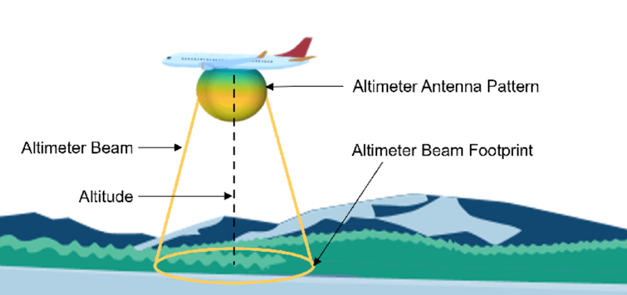
         Figure 1. Aircraft radar altimeter determining altitude above the terrain. ©2024 The MathWorks, Inc.

The altimeter can use either continuous waveforms or pulse waveforms. In this example, we will use a triangular FMCW waveform. Figure 2 shows the time frequency representation of such a waveform.

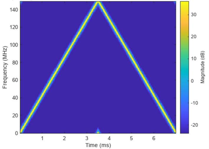Figure 2. Spectrogram of Altimeter Waveform BW = 150MHz and PRF = 143Hz. ©2024 The MathWorks, Inc

The altimeter antenna is modeled as a Gaussian antenna for illustration purposes. It is a common pattern used to represent a narrow beam and is parameterized with a 3 dB beamwidth. In this example, the 3dB beamwidth is set as 40 degrees, as shown in Figure 3.

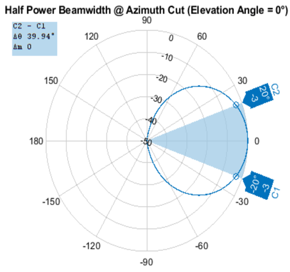
Figure 3. Power Pattern (dB), Broadside at 0.00° @4GHz. ©2024 The MathWorks, Inc.

The main parameters of the altimeter are captured in the following table. These parameters were derived from a common altimeter configuration found in the ITU document. 

Table 1. Altimeter configurable parameters.

Putting everything together, we can use a radar transceiver to simulate the altimeter.

A radarTransceiver from the Radar Toolbox is used to model the altimeter with the parameters discussed in the sections above.

 altimeterTransceiver = 

  radarTransceiver with properties:

                Waveform: [1×1 phased.FMCWWaveform]

             Transmitter: [1×1 phased.Transmitter]

         TransmitAntenna: [1×1 phased.Radiator]

          ReceiveAntenna: [1×1 phased.Collector]

                Receiver: [1×1 phased.ReceiverPreamp]

      MechanicalScanMode: 'None'

      ElectronicScanMode: 'None'

        MountingLocation: [0 0 0]

          MountingAngles: [0 -90 0]

    NumRepetitionsSource: 'Property'

          NumRepetitions: 2

The mounting angle is set to [0 -90 0] so the altimeter is facing the ground. 

Scene Creation

Next, we need to incorporate the altimeter into a simulation scenario. The simulation consists of a landing airplane over a land surface. To define such a simulation scene you can use the radar scenario tutorial with the Radar Toolbox. We start by defining the time span and the update rate of the scene. 

scene = radarScenario('StopTime',tStop,'UpdateRate',fUpdate)

Then we will mount the altimeter on the airplane and add the airplane into the scene.

altimeterPlatform = platform (scene, ‘Sensors',altimeterTransceiver,'Trajectory',landingFlightTrajectory);

The variable landingFlightTrajectory contains the airplane’s landing path.

Finally, let us define the ground surface. The ground surface of interest consists of both the terrain information, captured in surfaceHeight variable, and the reflectivity information, contained in the refl variable, that defines how strong the reflected signal is from the given location in the surface. In a radar system, the reflection from the ground is often termed as ground clutter. To many radar systems, the ground clutter is something they want to get rid of. However, for an altimeter, the ground reflection is all it looks for. Elevation data is loaded to generate the surface in the boundary of interest. The reflectivity of the land is created using an APL model which supports a 90-degree grazing angle in an urban environment. The coordinates of the flight trajectory are used to choose the boundaries of the surface. A LandSurface and ClutterGenerator are added to the radarScenario to generate IQ data of the ground reflection as the simulation progresses.

surface = landSurface(scene,'Terrain',surfaceHeight.','RadarReflectivity',refl);

clutter = clutterGenerator(scene, altimeterTransceiver);

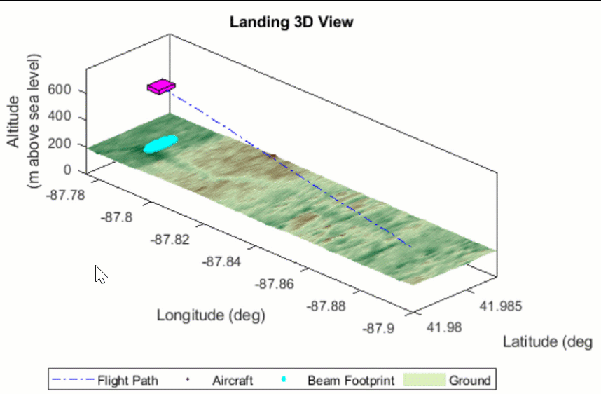The entire scene can be described by Figure 4.Figure 4. Aircraft landing 3D view. ©2024 The MathWorks, Inc.

Scene Simulation

To simulate the radar altimeter signal over time, we need to do two things. First, at each moment, we need to update all sensors and targets in the scene based on their trajectories. This is done by calling the advance() method of the scene. Then, we can use the receive () method of the scene to simulate the received signal of the radar altimeter at that moment. This process can be realized using a very simple simulation loop, as shown below.

while advance(scene)

    iqsig = receive(scene);

end

The simulation loop automatically moves the airplane following its trajectory, at an interval defined by the update rate, until the specified simulation stop time. The received signal at the altimeter is captured in the iqsig variable. Range response of a typical return from ground reflection looks like the following in Figure 5.

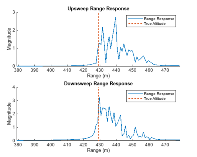Figure 5. Returned energy from an altimeter. ©2024 The MathWorks, Inc.

The leading edge of the signal would be a good indication of the altitude. To identify the leading edge, we apply a smallest-of CFAR detector to the signal and choose the first detection, as shown in Figure 6.

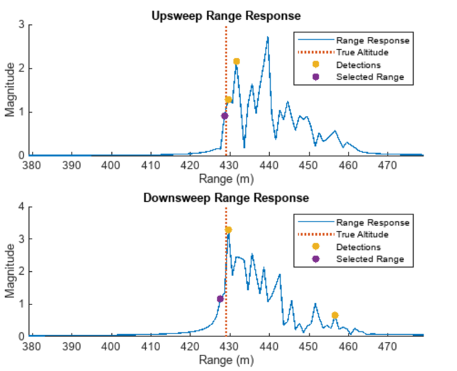
Figure 6. Range response of the signals in addition to the detections output from CFAR algorithm in the signal processor. ©2024 The MathWorks, Inc.

Note that in this example, we use a triangle sweep FMCW signal in the radar altimeter. This allows us to process up-sweep and down-sweep separately, as shown in previous figures, and then use the average of estimated altitude between the up-sweep and the down-sweep to be the final estimate of the altitude. This process provides a more robust estimate of the altitude by cancelling out the estimation error caused by Doppler.

The landing scenario measures the ability of the altimeter model to continue to produce good results as the range spread of the clutter return and the power level of the return vary. At higher altitudes, the return occurs over a much wider range and lower power level than at lower altitudes. Intuitively, the higher the aircraft in the air, the larger the error of the altitude estimate. This is because the echo from the ground is weaker at higher altitudes. This can be seen if we plot the returns received at the highest and lowest simulation altitudes. 

At lower altitudes, the range response is narrower and higher power. Despite this, the measurement error stays relatively stable throughout the aircraft’s descent due to the detection algorithm that was used. The accuracy limit requirements become more stringent with lower aircraft altitudes. The aircraft meets those measurement error requirements throughout the simulation scenario as seen in Figure 7.

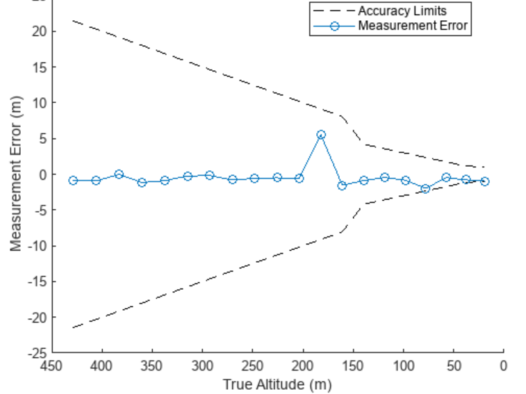
Figure 7.  Measurement error plot post simulation for landing trajectory. ©2024 The MathWorks, Inc.

From Figure 7, the estimation error is always within the desired range during the landing process. We can also incorporate the true altitude information into this curve, as shown in Figure 8, to provide a more intuitive look on how much error is tolerated over the landing process. The performance of the altimeter design in the banking scenario can also be simulated easily to evaluate the requirements as in this case the aircraft rolls and the shape of the signal return changes.

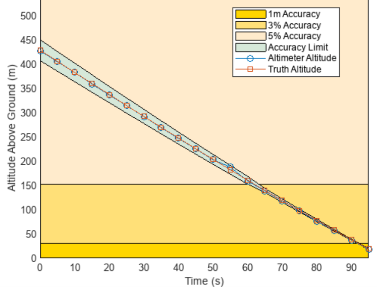
Figure 8. Measurement error plot post simulation for landing trajectory. ©2024 The MathWorks, Inc.

In this article, we showed how to simulate a radar altimeter in a landing scenario. The estimated altitude based on the received signal matches well with the true altitude. Therefore, this baseline simulation could be extended in the future to determine how radar altimeter performance is impacted by other factors in the environment, such as 5G interference. 

To learn more about the topics covered in this blog and explore your own designs, see the examples below or email me at abhishet@mathworks.com.