

Overview
In this part of the blog series, we continue to explore VRM output impedance curves in our power integrity challenges.
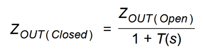
In the last part, we extracted the loop transfer function of our VRM on the bench, by measuring output impedance curves. However, there are additional ways to use the same output impedance to learn about the stability of our VRMs.
These are equations from the last post.
 Eq. 9-1
 Eq. 9-2
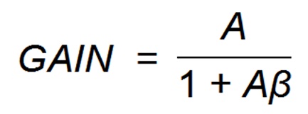
In any feedback loop system, stability of the loop is determined by the denominator in the form of ‘1 + T’ or ‘1 + Aβ when we have infinite gain as T or Aβ reach –1, making a division by zero.
Quality factor Q
Academically, this situation of the denominators producing a division by zero is evaluated as the quality factor Q, that is a peak, circled, as we can observe in the output impedance curves shown in Figure 1. The upper plots show the output impedance magnitude curves of this VRM, ON and OFF. The lower plots show the corresponding phase curves.
In these output impedance magnitude plots, curves of VRM=OFF are almost identical to the output capacitor response, as the regulator does nothing. The curve for VRM=ON shows a positive peak when crossing the plot of VRM=OFF highlighted with a green circle. This peak represents the amount by which ‘T’ or ‘Aβ’ come close to the ‘1’ in the denominator in the equations. The output impedance phase plots show a rapid phase shift at the frequency where we observe the magnitude peak.
In this part, we continue to use the same QSPICE™ simulation deck from the last part that is available at Qorvo repository on GitHub. There, the PyQSPICE module, written in Python, handles all the data arrangements, calculations and plotting and those operations are recorded in a session file by using a Jupyter Lab. You can modify the schematic and repeat the same plotting from this Jupyter Lab notebook.
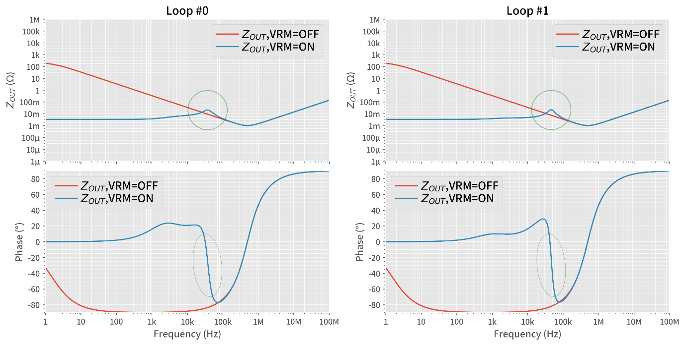
Figure 1: Gain and phase plots showing amplitude peaks and rapid phase changes when T or Aβ reach –1 in the equations noted
 Eq.9-3
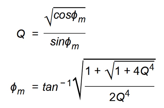
It is very important to note that this equation shows the reality of linking Q and Φm. The equation is never used in the following steps. Please carefully follow the procedure in the Python session file. These equations do not count the major component ESR of output capacitors, which plays a dominant role in output impedance analysis.
Nyquist diagram, stability margin
I want to emphasize that many power engineers blindly believe that a VRM with good phase and gain margin must be very stable. We can artificially design a VRM with very poor loop stability while having good phase and gain margin. Some actual designs fall into this category. Good phase and gain margin only guarantees that the VRM won’t oscillate.
To understand this statement, let’s review another powerful technique for visualizing stability - the Nyquist diagram, named after Dr. Harry Nyquist.
From the simulation deck, we can plot our Nyquist diagrams of loop #0 and #1 shown in Figure 2. The upper plots zoom-in around the origin and the lower plots are the full shape of the diagrams.
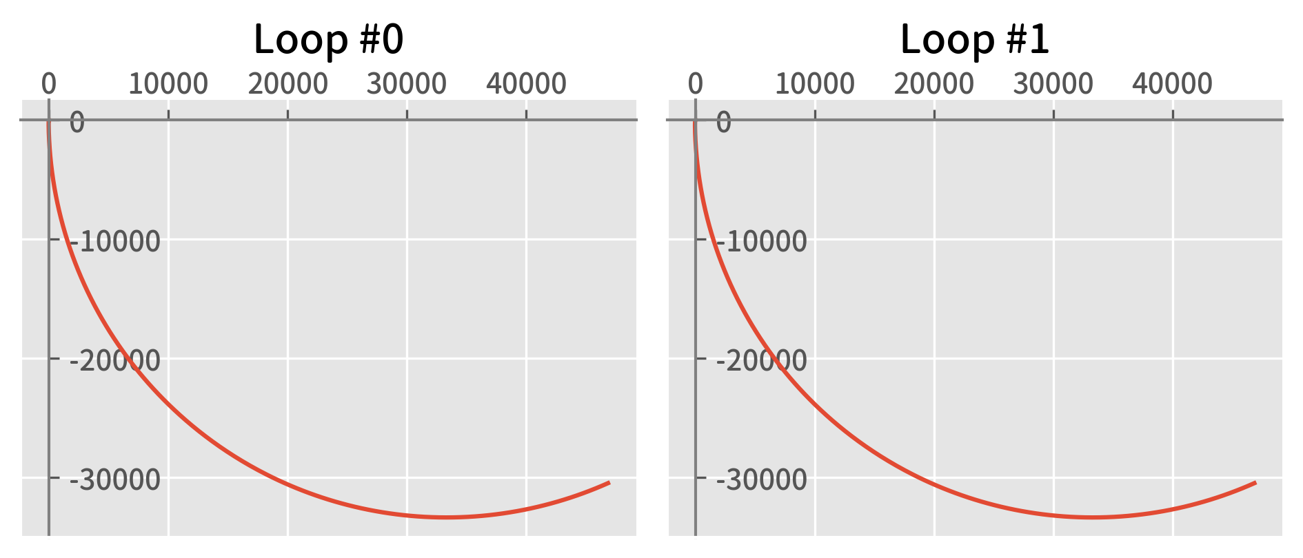
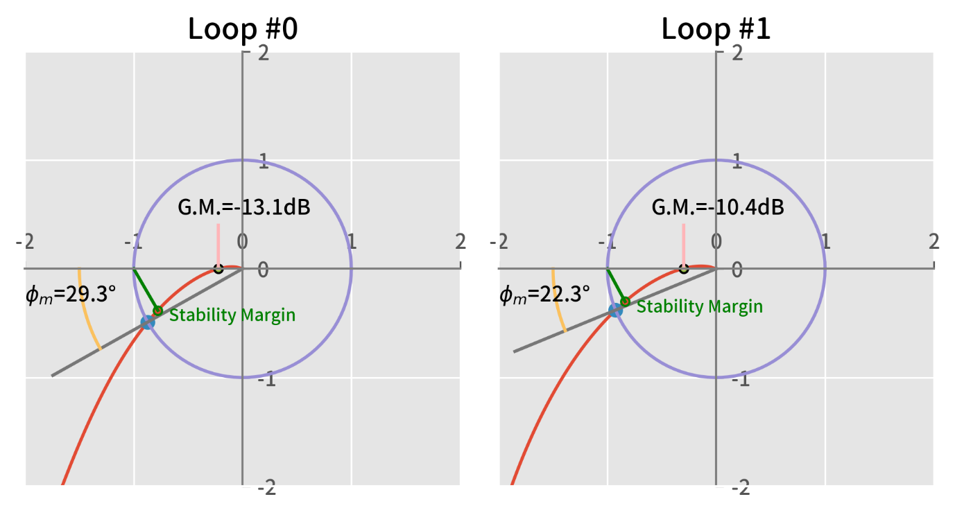
In the zoomed plots, phase and gain margins are marked.
Phase Margin | Gain Margin | |
Loop #0 | 29.3° | –13.1dB |
Loop #1 | 22.3° | –10.4dB |
NISM, non-invasive stability measurement
From this point, we follow the procedure of NISM, Non-Invasive Stability Measurement, from picotest.com.
Many engineers struggle with VRMs and evaluating their stability of their control loop for the following reasons:
- There’s no on-PCB feedback resistor to insert perturbation signals
- There’s no way to access the signal due to too high integration
- It becomes unstable, when inserting perturbation signals, no matter how small the perturbation signal is
- …and so on…
However, in all these situations, we can measure output impedance, as long as we can access the output capacitor of my VRM under test.
NISM 1st Step: peak of ZOUT @ VRM=ON
The first step is to measure a frequency point that gives a positive peak in the output impedance curve with VRM = ON.
In the simulation deck, we can get those points as shown below at the crossing ‘hairlines’ at the peaks. These are the frequency points of stability margin, corresponding to the green markers in our Nyquist diagrams above.
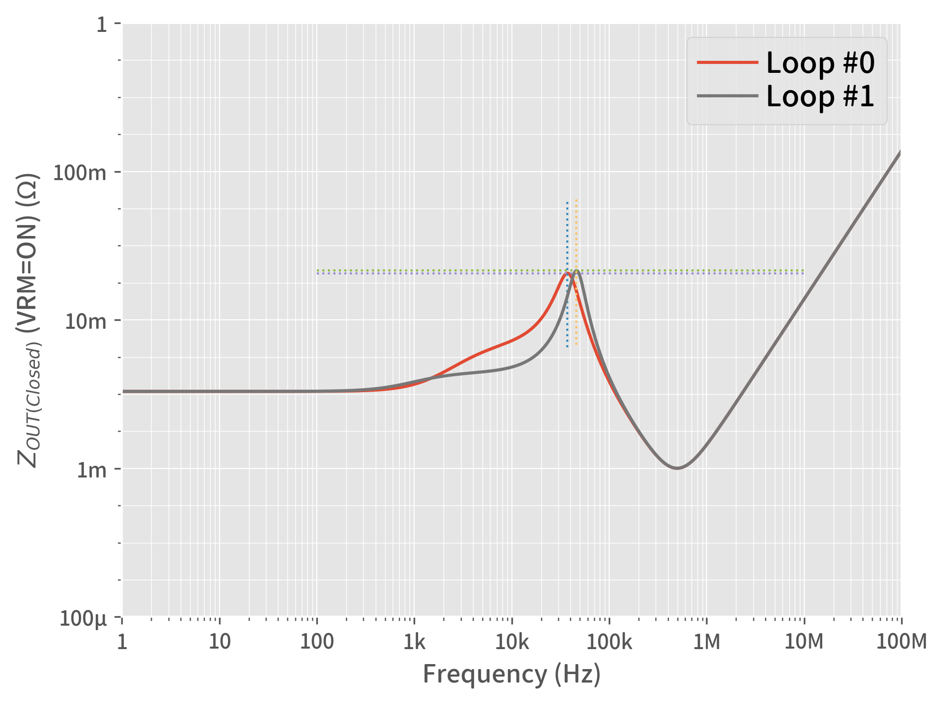
From this plot, by following the basic definition of quality factor Q from the equation Eq.9-4 below, we have an option to extract Q directly which we will not pursue due to many possible error factors expected from the dynamic Q shape on our output impedance curve.
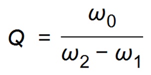 Eq .9-4
Where:
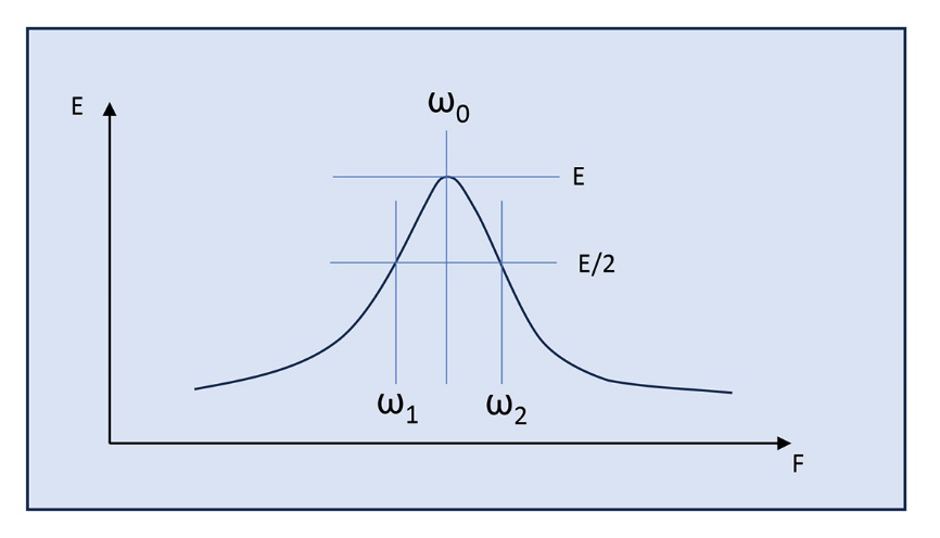
ω0 = Peak frequency
ω1 = Frequency that provides half the energy (-3 dB) of ringing, where ω1 < ω0
ω2 = Frequency that provides half the energy (-3 dB) of ringing, where ω0 < ω2
These are indicated in Figure 4.
However, there is a more sophisticated way to get Q.
NISM 2nd Step: Q(Tg) quality factor based on group delay
The second step is to generate the Q(Tg) curve that is a derivative of the output impedance phase curve. This procedure observes how quickly the phase changes within the green circles in the Figure 1. This step uses the fact that a phase curve of any phasor data re-generates the Q shape matching its amplitude curve.
This is not academically very precise, but allows us to extract a normalized, clean Q shape. This step works on any type of transfer function showing a Q shape, for example:
- Output impedance when the VRM is ON
- LC filter resonance
- Closed loop gain peak around its center frequency
Equations Eq.9-5 provide the procedure to follow on our output impedance phasor data.
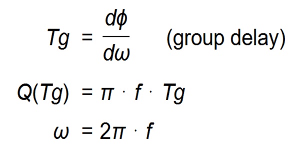 Eq. 9-5
In the simulation deck, we can obtain this clean Q shape plot where we can easily get the positive peak information of the frequency and value on the Q(Tg) curves, indicated by the crossing hairlines (Figure 5).
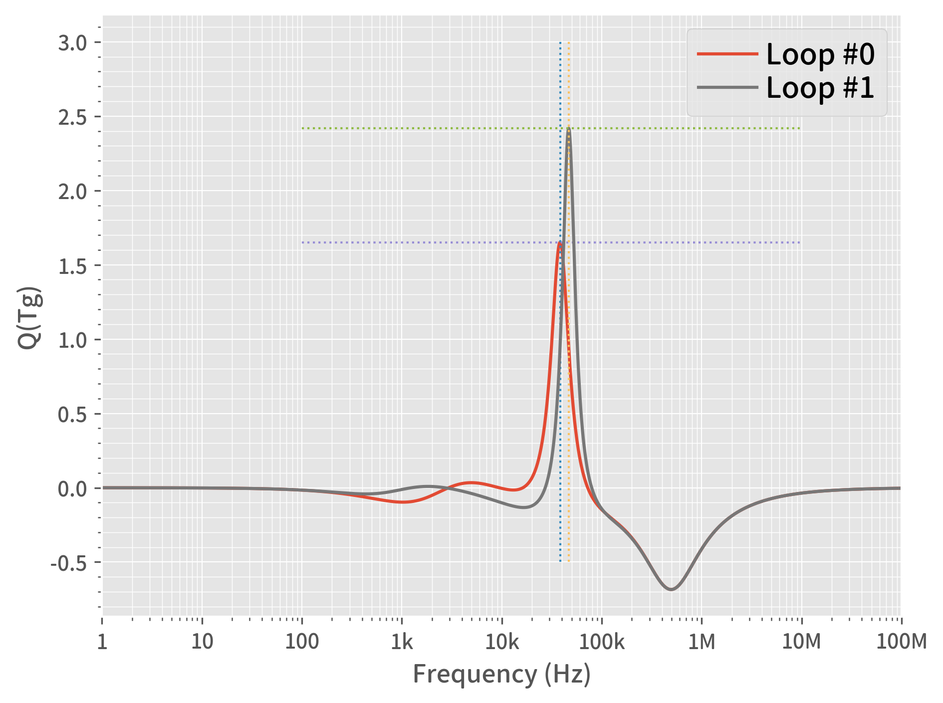
Frequency of ZOUT Peak | Frequency of Q(Tg) Peak | Q(Tg) Peak Value | |
Loop #0 | 37.180 kHz | 38.370 kHz | 1.651 |
Loop #1 | 46.138 kHz | 46.766 kHz | 2.418 |
NISM Final Step: Executing the NISM Program
The last step is to run a NISM calculation program, which is available from the NISM webpage on picotest.com, at no cost. We can find the detail of this NISM program in its earlier versions but the latest version provides much more accurate results. It is proprietary to Picotest and only available as a ‘black box’ engine.
By inputting the peak information from the first and second steps, we can get the NISM answer for phase margins, compared with our Bode plots.
Phase Margin from Bode Plot | Phase Margin from NISM | |
Loop #0 | 29.3° | 31.5° |
Loop #1 | 22.3° | 22.4° |
Note that in this simulation example, we can access various methods to evaluate loop stability. The NISM values come from actual bench measurements which would be difficult to obtain for a Bode plot.
We know that the NISM is very accurate when the loop has two poles. In our ideal simulation model, an ideal two pole model will never cross the 180° degree phase shift point as long as we model the ESR of the output capacitor, resulting in a non-textbook shape of Nyquist diagram. Furthermore, to illustrate two different loops, loop #0 has more complex poles that make it very different from a simple two-pole model. As a result, we can treat our loop #1 as ‘more like’ a two-pole system and the NISM result for loop #1 matches the Bode plot better than loop #0.
This difference for loop #0 can be observed in the Nyquist diagram. We can see that the loop #0 Nyquist curve reaches the (–1, 0) point closer than the loop #1 does.
[1] Fundamentals of Power Electronics, 2nd Edition (Robert Erickson and Dragan Maksimovic, Springer Science+Business, 2001)
[2] Killing the Bode Plot (Steve Sandler, DesignCon, Jan 2016)