Harmonic Load Pull with High Gamma Tuners

Microwave power devices, widely used in modern wireless and communications systems, must operate in a nonlinear mode in order to operate efficiently. Nonlinear operation means that the only valid way to test them is under actual operating conditions of DC bias, RF power and impedance. Small-signal S-parameters are not sufficient.

Because of the need to control impedances seen by power devices, load pull has become a primary method for characterizing active RF and microwave devices. Load pull systems generally include tuners for impedance control, in addition to whatever equipment is needed for the stimulus and measurement of the Device Under Test (DUT). Typically, whatever can be measured in a matched environment, such as 50 Ω, can then be measured as a function of impedance.

Some general applications of load pull include: process development, where load pull measurements are used to determine the effects of varying process parameters; direct amplifier or oscillator design, where load pull measurements are used to determine the optimum source and load impedances that can then be synthesized with matching networks using a linear simulator; large-signal device modeling, where load pull data is used to adjust device models to make them more accurate; production, where the tuners typically set specific load and source impedances for a single measurement on-wafer; and ruggedness testing of modules, where the device is measured with a specified output VSWR at all phases.

Types of Tuners

Most load pull systems use passive tuners to control impedance. These tuners may be mechanical or solid state. Mechanical tuners use motors to move mechanical parts to change the impedances, while solid state tuners typically use switch elements, such as PIN diodes, to select from a fixed set of impedances.

The most common tuner type in use today is the mechanical slide screw tuner. For coaxial tuners, it typically uses a 50 Ω slab line, consisting of two parallel ground planes with a center conductor. When the mismatch element, called a probe, is far from the center conductor, the slab line acts like a very good, low-loss, 50 Ω TEM transmission line. As the probe is moved toward the center conductor, the mismatch smoothly increases until it reaches a maximum when the probe is close to the center conductor. Phase of the mismatch is varied by moving the probe parallel to the center conductor.

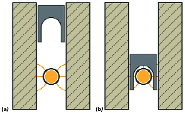
A cross-section of a typical mismatch probe is shown in Figure 1. Figure 1a shows the probe far from the center conductor, where it has no effect on the fields, resulting in a good 50 Ω transmission line. Figure 1b shows the probe at the opposite end of its travel, close to the center conductor. In this position, it interferes with the electrical fields, producing a large mismatch. As the probe is moved between these two extremes, the mismatch magnitude is varied smoothly.

Ideally the probes should be non-contacting, touching neither the ground planes nor the center conductor. This enables the motors to move the probes very quickly with no perceptible wear or change over time. This provides long tuner life, excellent repeatability, and saves time because a single calibration is often good for a long time, even years. Some mechanical tuners use probes that make sliding contact to connect the probe with the ground planes. Contacting probes are easier to design, but at the cost of shorter tuner life, slower operation and poor repeatability.

The High Gamma Tuner

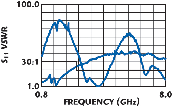
The traditional slide screw tuner probe has a frequency response similar to a low impedance line section that is one quarter-wave long at the center frequency. The maximum available mismatch peaks at the center frequency, and drops off on either side. So if the specified bandwidth is narrow, fairly high matching is available. If a wider bandwidth is specified, then at the band edges, the available matching range will be reduced. The measured response of one model tuner of this type is shown in Figure 2. In this case, there is a low frequency probe and a high frequency probe. Only one probe is used at a time, depending on the frequency of operation. The maximum VSWR vs. frequency of the two probes are overlaid on the plot to show the overall matching range vs. frequency for the two-probe tuner. This matching range is adequate for many applications where the fixture losses are low.

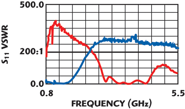
The frequency response of the High Gamma Tuner (HGT) is dramatically different. An HGT is shown in Figure 3, and a typical HGT response is shown in Figure 4. This tuner produces an extremely high mismatch over its entire frequency band, also with low and high frequency probes. Of course, as the probe is retracted away from the center conductor, the mismatch reduces very smoothly until the tuner again looks like a very good 50 Ω line. The probes are non-contacting for long life and good repeatability.

The high matching range of the HGT is very helpful in overcoming losses in a fixture or wafer probe. This has opened the door to on-wafer measurement of 35 dBm power devices,¹ since the high matching range allows matching of the low device impedance. This saves a tremendous amount of turn-around time and expense during device design and production stages. The high matching range of the HGT over its full band is also very effective in harmonic tuning.

Introduction to Harmonic Tuning

Harmonic load pull consists of controlling the source or load impedance at a harmonic of the fundamental frequency. For example, if the DUT operating frequency is 2 GHz, then harmonic load pull might vary the impedance at the second harmonic, which is 4 GHz. The measured data would still be at the fundamental frequency, but the harmonic load pull would show the effect of the harmonic impedance on the fundamental frequency operation.

Harmonic load pull primarily affects efficiency and linearity parameters. Efficiency is usually computed as power-added efficiency, which is the ratio of RF power added by the DUT divided by the DC power into the DUT. Linearity is measured with a variety of parameters, including two-tone intermodulation, ACPR, ACLR, EVM, PM/PM, or AM/PM. All of these parameters show how the performance changes as a function of power level.

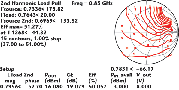
An example of harmonic load pull data is shown in Figure 5. This is a plot of efficiency at the fundamental frequency vs. the second harmonic impedance. All other variables, including the DC bias, RF input power and fundamental impedances were held constant. There are 14 contours plotted, with each contour representing a one percent efficiency change, so the harmonic impedance changed the efficiency by over 14 percent. The worst efficiency is in the upper right part of the Smith chart, and the best efficiency is in the lower part of the chart. Note that efficiency is not very sensitive to impedance in the area of the chart that gave the best values.

In amplifier design, efficiency and linearity parameters often produce a conflicting trade-off. Higher efficiency may come with worse linearity, and vice versa. Harmonic load pull will often find impedance combinations that will allow both to improve together.

Harmonic load pull is really only useful when the fundamental impedance is already tuned up fairly well. If the fundamental impedance is off, then the DUT will not be operating very well, and the harmonic impedance will not matter. Also, DUT operation is typically very sensitive to the fundamental impedance, so it is important for the harmonic tuning to be independent of the fundamental impedance. Without this tuning isolation between the harmonic and fundamental impedances, the resulting data may not be meaningful.

Harmonic load pull is also only useful when the DUT is operating in a nonlinear mode and generating harmonic energy from the fundamental frequency input. The data in Figure 5 was taken with the DUT somewhat saturated. In back-off operation, the harmonic load pull may have less effect. Nevertheless, this shows that harmonic tuning is an important tool for optimizing DUT performance.

Most of the time, the best harmonic impedance will be at the edge of the Smith chart. There are exceptions, but power delivered at the harmonic is generally undesirable, so it should be all reflected back to the DUT at an appropriate reflection phase to allow the signals to recombine advantageously. In that case, a harmonic tuner that tunes only at the edge of the Smith chart may be sufficient to show the best reflection phase to optimize the DUT operation. However, as shown in Figure 5, tuning over the entire chart may give insight about tuning sensitivities. Also, even if losses limit the harmonic reflection magnitude, the measurement is still quite useful because the best phase can still be clearly seen.

Harmonic Tuning Methods

There are several methods of harmonic tuning. Some of the most common methods of passive tuning include the Fixed Impedance method, the Multiplexer method, the Cascaded Tuner method and the Stub Resonator method. No single method is perfect, as there are benefits and weaknesses to each method. The best method depends on the specific needs.

The Fixed Impedance method consists of putting a fixed harmonic circuit into a fixture. Often this might be just a shunt stub that reflects all the harmonic energy at the desired phase. This method is not exactly harmonic load pull, since it is not tunable, but it does control the harmonic impedance and it is simple and widely used in fixtured measurements.

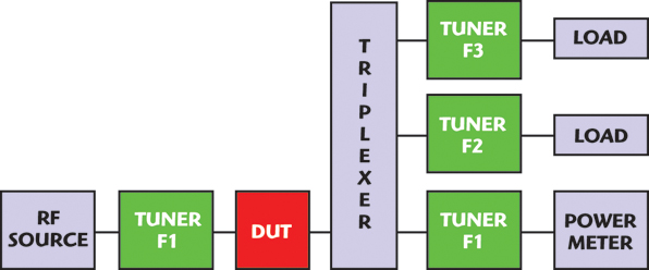
The Multiplexer method, as shown in Figure 6, uses filters to separate the fundamental and harmonics. A triplexer has three filters. One path passes the fundamental and blocks all harmonics. The second path passes the second harmonic and blocks the fundamental and third harmonic. The third path passes the third harmonic and blocks the fundamental and second harmonic. Three separate tuners are used, each tuning only one harmonic (or fundamental) because that is the only energy that it sees.

The biggest benefit of the Multiplexer method is excellent accuracy due to very high tuning isolation between harmonics. This comes because the frequency separation between harmonics is fairly wide, so good isolation is easy for the filter designers. This method also provides uniform tuning over the entire Smith chart at each harmonic. This method is widely used, since these benefits have made it the method of choice for many applications. The disadvantages of the multiplexer approach include the need for a multiplexer for each band, since it is necessarily band limited. It also requires a more complex bench layout and has multiple outputs, which complicates some measurements. The multiplexer also has some loss, which reduces the tuning range by a small amount.

The Cascaded Tuner method, as shown in Figure 7, combines positions of multiple cascaded tuners. For example, if the two cascaded load tuners in Figure 7 are both characterized at 1000 positions, then there are 1,000,000 possible combinations of characterized positions available. If all the combinations producing the same fundamental impedance are selected, a wide variety of harmonic impedances will be produced by those combinations. Measuring the DUT with the selected combinations would then be a harmonic load pull with the fundamental impedance held constant.

Two cascaded tuners produce two degrees of freedom, so the fundamental and the second harmonic may both be tuned independently, or the fundamental and the third harmonic may both be tuned independently. Three cascaded tuners produce three degrees of freedom so that the fundamental, second harmonic and third harmonic may all be tuned independently.

The benefits of the Cascaded Tuner method include the fact that no band limiting component is needed. The only limitation is the response of the tuners themselves. Also, the matching range is helped by not having a component between the DUT and tuners. In addition, it uses a fairly simple bench layout, with only one output. A disadvantage of the Cascaded Tuner method is limited tuning isolation. When multiple combinations are selected to give the same fundamental impedance, it is really the same impedance within some tolerance. So a harmonic load pull also moves the fundamental impedance a little bit. Since the DUT performance is usually very sensitive to the fundamental impedance, it may be hard to separate the effects of moving the harmonic a lot vs. moving the fundamental a little. However, this problem may be overcome by constraining the harmonic impedance during a final fundamental load pull, since the harmonic is usually less sensitive.

The Stub Resonator method is shown in Figure 8. The first tuner reflects all the third harmonic energy with a controllable phase. The second tuner reflects all the second harmonic energy with a controllable phase. The third and final tuner then is a normal tuner to tune the fundamental frequency.

The two harmonic tuners each consist of two shunt open stubs that are one quarter-wave long at the particular harmonic. This reflects all that harmonic energy back to the DUT, and the reflection phase is controlled by sliding the stubs along the center conductor. The stubs connect to the center conductor with a metal spring.

The benefit of the Stub Resonator method is a fairly simple bench layout. There are some major disadvantages to the Stub Resonator method. It has very poor tuning isolation. Tuning the harmonic has a fairly significant effect on the fundamental impedance. This problem can be reduced by re-tuning the fundamental after the harmonics are set, but the poor isolation may require multiple iterations. It is very narrow band—separate resonators are required for every frequency, and the tuners must be recalibrated when the resonators are changed. The sliding contacts may work fairly well when new, but tend to become unreliable after some use the loss of the harmonic tuners limits the tuning range of the fundamental tuner.

Harmonic Tuning with the High Gamma Tuner

The low loss and high matching range of the HGT make it an ideal tuner for use with the Cascaded Tuner method of harmonic tuning. Figure 9 shows a software Tuning Control Panel with the Cascaded Tuner method of Figure 7 selected for harmonic tuning. The Position Control block shows the physical tuner positions. The Reflection Control block shows or sets the target gamma for each harmonic. Markers on the Smith chart show the actual gamma produced by the current combination of tuner positions. Marker 1 shows the fundamental gamma, and marker 2 shows the second harmonic gamma.

For this setup, the load pull operator would enter a target magnitude and phase for both the fundamental and second harmonic gammas in the Reflection Control block. Clicking on “Move Reflection” would then move the tuners and update the entries to show the actual gammas achieved. Alternately for this setup with two tuners, the fundamental and third harmonic could be controlled.

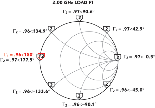
Figure 10 shows an overlay of several Smith charts from the Tuning Control Panel. It shows the markers as the second harmonic gamma is swept around the edge of the Smith chart in 45° increments. During this second harmonic tuning sweep, the fundamental gamma remained constant at 0.96 magnitude with 180° phase. The magnitude of the second harmonic gamma was either 0.96 or 0.97 at every phase angle around the Smith chart. This high gamma at every phase combination for both the fundamental and harmonic impedances is only possible with the High Gamma Tuners. This provides an excellent solution for testing low impedance power devices.

Summary

Load pull is necessary to test non-linear power devices. Harmonic tuning consists of controlling the harmonic impedance independent of the fundamental impedance as seen by the DUT. High Gamma Tuners provide a much higher matching range as compared to traditional mechanical tuners, and the high matching range applies to the entire operating bandwidth. This is very useful for matching high power devices that have very low impedances, especially with the losses of a fixture or wafer probe.

Harmonic tuning is useful to improve efficiency and linearity of non-linear power devices. In most cases, it is desirable to set the harmonic impedance to a high reflection, and just select the right phase to get the best DUT performance at the fundamental frequency. There are several methods of harmonic tuning that have been used in the industry, but the Cascaded Tuner method when used with High Gamma Tuners provides some of the best performance available. Very high gammas are available for both the fundamental and harmonic impedances at any phase combination.