Mixer Spur Analysis with Concurrently Swept LO, RF and IF: Tools and Techniques

Assessing mixer spurs reliably can enable first-cut success in communication hardware design with reduced development time and product cost. The tools used to determine these spurs must be able to manipulate LO, RF and IF frequencies concurrently over their continuous bandwidths. These tools can be either standard graphical charts or specific computer software.

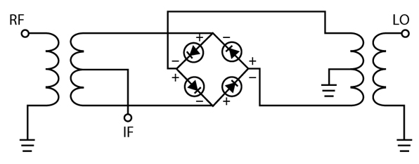
The graphical chart shown in Figure 1 can be used to estimate the spurs within all three bands combined and extrapolate the specifics of each spur. A new JAVA applet (advanced) available on Hittite Microwave Corp.’s Web site, http://www.hittite.com, under the Product Support section, can be used to perform intricate spur calculations in seconds. The calculations include the spurs’ bands of incidence in LO, RF and IF concurrently, and their suppression levels in a double-balanced mixer (Figure 2). Both of these methods of spurious analysis are discussed in this article. Furthermore, the equations related to the spurious analysis are derived and explained, including construction of the spur lines, bandwidth apertures (windows) and determination of the incident spurs within the concurrently swept LO, RF and IF bands.

Graphical analysis involves drawing a rectangular aperture (window) on the frequency ratio spur chart. The spur lines encountered within the aperture (associated with a specific LO frequency) fall inside the RF and IF operating bands. The intercept points of a specific spur line within the perimeter of the aperture determine the RF and IF frequency band segments involved. The ratio spur chart illustrates the spur analysis for a double-balanced mixer downconverter. In this example, the input RF range is 15 (RF_LOW) to 18 GHz (RF_HIGH), the LO is 10 GHz and the output IF range is 5 to 8 GHz. In addition, a bandpass filter is used at the output to limit the IF between 6 (IF_LOW) and 8 GHz (IF_HIGH). With these frequency parameters, one can draw a rectangular aperture (blue rectangle), as shown. The coordinates (x, y) of the four vertices of the aperture are: 1.5 (RF_LOW/LO), 0.6 (IF_LOW/LO); 1.5 (RF_LOW/LO), 0.8 (IF_HIGH/LO); 1.8 RF_HIGH/LO), 0.6 (IF_LOW/LO); and 1.8 (RF_HIGH/LO), 0.8 (IF_HIGH/LO). The spur lines encountered within the aperture, R-L, 2R-3L, 3R-4L and 4L-2R, fall in the RF and IF operating bands. Beware that not all possible spurs are shown in this chart.

The spur line labeled R-L incident within the aperture, of course, represents the desired IF output. The RF and IF frequency ranges where this R-L spur occurs can be deduced from the spur’s intercept points with the perimeter of the aperture. In this particular case, the coordinates in the Ratio Chart — (RF/LO)₁ = 1.6, (IF/LO)₁ = 0.6 and (RF/LO)₂ = 1.8, (IF/LO)₂ = 0.8 — can be multiplied with the LO frequency, 10 GHz, to obtain the RF range 16 to 18 GHz, and the IF range 6 to 8 GHz. Similarly, other spurs of interest can be treated in this way to find their RF and IF frequency range of incidence.

The concept of spur apertures (windows) just described can be extended to include spurs within a range of LO frequencies. Again referring to the ratio chart, another aperture (the orange rectangle) can be drawn for an LO frequency of 12 GHz. In order to encompass all the spurs within the LO frequency range of 10 to 12 GHz, connecting lines can be simply drawn between the corresponding vertices of the two apertures (yellow dashed lines). The spur lines observed within the 3D-like figure bounded by the two apertures (associated with LO = 10 GHz and LO = 12 GHz) and the connecting lines are incident with the concurrently swept LO, RF and IF bands. Notice the R-L line from the first aperture (with LO = 10 GHz) continues and intercepts the second aperture (with LO = 12 GHz) at its bottom-right corner, creating a new set of intercept coordinates ((RF/LO)₃, (IF/LO)₃; (RF/LO)₄, (IF/LO)₄). In this particular situation, the R-L spur intersects a vertex, generating only one new intercept point, (RF/LO)3 = 1.5, and (IF/LO)3 = 0.5, leading to single RF and IF frequencies of incidence.

As described previously, to obtain the true frequencies, the ratio chart coordinates of the R-L spur must be multiplied with an LO frequency of 12 GHz. This generates RF = 18 GHz (1.5 × 12 GHz) and IF = 6 GHz (0.5 × 12 GHz). It can be deduced that as the LO increases from 10 to 12 GHz, the desired R-L spur incidence bandwidth decreases from an RF of 16 to 18 GHz and an IF of 6 to 8 GHz to a single RF of 18 GHz and a single IF of 6 GHz.

Similarly, an LO frequency range of incidence can be assessed for a particular spur. For example, the spur line 2R-2L intersects the connecting dashed line at RF/LO = 1.364, which corresponds to RF = 15 GHz (RF_LOW) and LO = 11 GHz, and continues on to intersect another connecting line, which corresponds to RF = 15 GHz (RF_LOW) and LO = 12 GHz before it completely exits the 3D-like figure. The LO frequency span, 11 to 12 GHz, is the minimum range over which this spur is incident. In order to ensure that, for a particular spur, all bands of incidence are accounted for within the LO bandwidth, the intercept points with the other connecting, dashed lines must be computed. These techniques can also be applied to analyze spurs for an upconverter. The left portion of the chart can be used for a lower sideband upconverter. Figure 3 shows an upconversion chart incorporating both lower and upper sideband spur lines.

In order to alleviate the burden of the manual process previously described, a new JAVA applet (advanced) has been developed. The applet exhibits multiple functions and is versatile, performing complex spurious analysis with speed. The applet extends the concepts of the fixed LO frequency spurs developed by A. Roetter and D. Belliveau.¹ The new JAVA applet utilizes their mathematical and graphical techniques. The spur analysis results are presented in both tabular and color-coded graphical formats. The graphical area can be zoomed for finer details, and panned for overview of the analysis. A particular spur line can be mouse-selected to highlight its parameters in the table. Furthermore, the software facilitates spur power suppression calculations for a double-balanced mixer.²

Figure 4 highlights the software’s capability. It presents spur calculations referring to the example previously treated using a standard frequency ratio spur chart. The rectangular aperture on the right in the spur plot represents an LO of 10 GHz; its corresponding true RF and IF frequencies are depicted on the bottom x-axis and left y-axis, respectively. The aperture on the left represents an LO of 12 GHz, and its true RF and IF values are shown on the top x-axis and right y-axis. It is apparent that both apertures depict the same RF and IF frequency bands. However, the spur content in each aperture is different due to its specific LO frequency. The dashed lines joining the two apertures depict the LO-axis sweeping from 10 to 12 GHz. The spur lines incident within this 3D-like figure occur concurrently in parts of the LO, RF and IF bands. The spur line intercept points with the edges of the 3D-like figure can be used to assess the corresponding segments of the LO, RF and IF bandwidths.

The table adjacent to the chart lists the parameters associated with the spur lines displayed on the plot. This includes the spur index (m × n), whether it is in-band (in box), its dominating range of frequencies and its suppression in dBc. Furthermore, this information may be exported for use in Agilent ADS, or any other program that accepts tab-delimited text files.

The bottom portion of the spur plot is the Graphical User Interface that facilitates parameter inputs via various tabs. It also provides an option to select upconversion or downconversion. Once the inputs are entered, click the Calculate button using the mouse. The new applet also includes an eight-minute demo under the Help Button Menu, which highlights features perhaps not intuitive to the user.

Constructing Spur Lines

The basis for spur frequency calculations comes from two equations:

F_IF = ±mF_RF ± nF_LO (1)

F_RF = ±mF_IF ± nF_LO (2)

Equation 1 is used for the downconversion mode and Equation 2 for the upconversion mode. It can be observed that the RF (F_RF) and IF (F_IF) terms merely switch places in these two equations depending upon upconversion or downconversion mode. Hence, a general equation can be written as

F_OUT = ±mF_IN ± nF_LO (3)

In this equation, F_IN represents the input frequency into the mixer along with the LO frequency (F_LO) drive, and F_OUT represents the output frequencies generated by the mixer. The prevailing output frequencies can be the sum and difference products due to the F_IN and F_LO mixing. However, along with these products, the mixer also produces the sum and difference of all the higher order multiples, or harmonics, of the F_IN and F_LO frequencies. These multiples are represented by the coefficients m and n, and are used to identify each F_OUT spur. Generally, when upconverting, the desired output is a sum product with m and n values of 1; the equation F_RF = F_IF + F_LO represents the desired upconverted signal. When downconverting, the desired m and n coefficients are 1 and –1, respectively; the equation F_IF = F_RF – F_LO (the difference frequency) represents the desired downconverted signal. All other spurs are usually undesirable. These equations are adequate for spurious analysis when single frequencies are involved. However, when a range of frequencies is involved, Equation 3 must be graphed for every spur within the frequency band and with the desired coefficients.

When the LO frequency is fixed at a value, F_{LO_1} for instance, these equations transform into the equation of a line, y = mx + b. The parameter being swept is the input frequency (F_IN), which corresponds to x in the equation. The coefficient, m, of the parameter F_IN, is equal to the slope (dy/dx) of the line. The LO term (nF_LO) is represented by the constant b (a value, F_{LO_1}) in the line equation, the y-intercept. A set of spur line plots can be generated for several integer values of m with a common intercept point for n = 1. The process can be repeated for other sets of spur lines with different integer values of n. Each set differs only in the vertical offset of its intercept point, corresponding to different values of n.

The spur line concept developed for a fixed LO frequency (F_{LO_1}) can be extended to apply over a range of LO frequencies, F_{LO_1} to F_{LO_2}. By creating another set of spur lines for F_{LO_2} and shading the area between the corresponding F_{LO_1} spur lines and F_{LO_2} spur lines, one can represent the LO range F_{LO_1} to F_{LO_2}. However, in this article, a different approach (bandwidth apertures) is used to account for spurs with a swept LO.

Constructing Bandwidth Apertures with a Swept LO

A rectangular aperture can be drawn on a broadband spur chart created with the LO frequency F_{LO_1}. The horizontal and vertical sides of the aperture represent the bands of F_IN and F_OUT, respectively. The line equations of the aperture’s perimeter are given by x = F_{IN_1}, x = F_{IN_2}, y = F_{OUT_1} and y = F_{OUT_2}. Another aperture can be drawn on the same referenced spur chart (F_{LO_1} chart) for LO frequency F_{LO_2} with the aid of mathematical manipulation. The two apertures on the same chart provide the convenience of depicting the spurs incident within the LO bandwidth (F_{LO_1} to F_{LO_2}). It should be emphasized that the new length and width of the second aperture still represent the same F_IN and F_OUT frequency bands as in the first aperture; however, the x-axis and y-axis scales cannot be read directly as true frequencies for the second aperture.

In order to facilitate drawing of the second aperture, a mathematical transform of the vertices’ positions of the first aperture needs to be performed. The true frequency x-axis and y-axis scales need to be transformed into ratio scales, F_IN/F_LO and F_OUT/F_LO, respectively (similar to the ratio scales in the graphic spur chart). With the ratio scale axis, the coordinates for the second aperture can be generated using the LO frequency F_{LO_2}. Then those coordinates can be transformed to equivalent true frequencies that can map into the spur chart created using the LO frequency F_{LO_1}.

The following equations relate the specific values on the true frequency x-axis to the ratio x-axis:

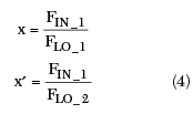
The ratio of the specific points on the ratio x-axis can relate to the LO frequencies as

Mapping x' (a ratio number), to (F_{IN_1})' (an equivalent true frequency), onto the true frequency spur chart associated with the LO frequency F_{LO_1}

(F_{IN_1})' = (x')F_{LO_1} (6)

With simple substitutions, an equation that lacks x and x' and only involves true frequencies can be developed. Substituting for x' in Equation 6 with Equation 5:

Substituting for x using Equation 4:

It is apparent by observing Equation 7 that (F_{IN_1})' can be mapped directly onto the true frequency spur chart associated with the LO frequency F_{LO_1}. Similarly, (F_{OUT_1})' can also be mapped. Rewriting Equation 7 in general terms yields

F_IN(F_{LO_1}/F_{LO_2}) = (F_IN)' (8)

F_OUT(F_{LO_1}/F_{LO_2}) = (F_OUT)' (9)

Using Equations 8 and 9, all vertices of the first aperture (associated with F_{LO_1}) can be transformed to construct a second aperture, representing spurs at the LO frequency F_{LO_2}. The corresponding vertices of the two apertures can be linked to form a 3D-like cubic figure, representing the full LO sweep range, F_{LO_1} to F_{LO_2}. All spurs encountered within the figure are incident in some segment of the band with regard to each of the LO, RF and IF frequency ranges. Be advised that the true frequency axis only corresponds to the first aperture associated with F_{LO_1}. The second aperture is associated with a different true frequency scale. However, the vertices of the second aperture do represent the same RF and IF frequencies as the respective vertices of the first aperture.

Spur Power Calculations

The equations used in double-balanced mixer spur power calculations involve gamma function and indefinite integrals. The specific algorithms and the JAVA code used for power calculations in this new applet (advanced) are described in an article by A. Roetter and D. Belliveau.² The accuracy constraints for the power calculations as described in this publication also apply to the new JAVA applet. The applet also facilitates specifying the characteristics of a diode ring, such as V_forward and imbalance between diodes, to handle specific cases of spur power calculations. The diode ring parameters involved are also explained in this publication.

Conclusion

The new JAVA applet (advanced) developed for mixer spur analysis supercedes the use of traditional spur charts in both functionality and speed. It can gracefully handle all three continuous (not discrete frequency steps) bands (LO, RF and IF) sweeping concurrently. The analysis results are presented in both tabular and graphic displays. The 3D-like cubic figure constructed with the apertures (windows) on the spur chart enable engineers to discern the vital spurs within the operating bands, and swiftly assess their impact on a system’s performance with confidence. The mathematical basis of the software algorithm has been explained, encouraging further work towards dual-mixer spurious analysis.

Acknowledgments

Daniel Gandhi wishes to thank David Belliveau for his inspiration throughout his high school years. (It should be noted that Mr. Gandhi is one of the youngest authors to ever publish a technical feature in Microwave Journal and should be congratulated).

References

1. A. Roetter and D.A. Belliveau, “Single-tone IM Distortion Analyses via the Web: A Spur Chart Calculator Written in Java,” Microwave Journal, Vol. 40, No. 11, November 1997.
2. B.C. Henderson, “Reliably Predict Mixer IM Suppression,” Microwaves and RF, Vol. 22, No. 12, November 1983.

Daniel Gandhi completed his senior year at Waltham High School (Waltham, MA) in the spring of 2002. He is currently enrolled at Brandeis University where he expects to major in physics and computer science. During his summer breaks, he has been working with the engineering group at Hittite Microwave Corp. since 2000.

Christopher Lyons received his BS degree in electrical engineering from the University of Lowell (now University of Massachusetts, Lowell) in 1982. From 1981 to 1983, he was with the Frequency Sources Division of Loral Corp. where he contributed to the development of MIC FET oscillators, amplifiers and control devices. In 1985, he joined the Special Microwave Devices Operation of Raytheon Co. where he developed numerous multi-function modules and sub-systems. In 1990, he worked in the Missile Systems Division of Raytheon in the development of a novel frequency-locked Ku-band noise degenerated oscillator for the Patriot program. In 1992, he joined the Mayflower Communications Co. where he was responsible for development of a multi-channel high performance GPS receiver front-end and frequency synthesizer. In 1993, Mr. Lyons joined Hittite Microwave Corp. as a principal engineer where he has been responsible for integrated MMIC assemblies and MMIC frequency synthesizer designs. He has also been responsible for the development of automotive radar sensors and has four US patents pending in that area.