A Phase Noise Analysis Tool for Sparse Numerical Phase Noise Data

This article describes a phase noise analysis tool that creates a numerical model from discrete phase noise data. The tool includes an adaptive algorithm to identify spurious deterministic components in the data. It also creates a physics-based numerical model for the random noise component.

Despite its apparent simplicity, analyzing the temporal and Fourier characteristics of an oscillator from its phase noise characteristic presents challenges to designers and those wishing to specify an oscillator for an application.¹ Frequency spurs in the characteristic, measurement noise and a limited number of measured data points can significantly impact the accuracy of random and deterministic jitter components. To alleviate these difficulties, a phase noise analysis tool has been developed for use with measured or simulated phase noise data. Unlike other online and commercial phase noise analysis tools^2-5 that compute an integrated jitter value independent of the nature of the phase noise characteristic, this tool creates a numerical random noise model based on physical phase noise mechanisms to yield a more precise analysis. The tool algorithmically identifies and quantifies deterministic frequency components, which are removed to create the final model. The model makes the slope visible as a function of offset frequency to easily identify the physical nature of its noise components. The random and deterministic jitter components are computed using a bandpass filter with user-defined highpass and lowpass 3 dB corner frequencies. Computation of the jitter components using a brick-wall filter, a first-order filter or both is supported. Output data is provided in both graphical and tabular formats.

RANDOM PHASE NOISE NUMERICAL MODELING

Phase and Frequency Noise Sources

The sources of phase and frequency noise, although well recognized in measurement, are not fully understood.^6-8 The two most prevalent noise mechanisms are thermal noise and 1/f noise. The former represents Johnson noise, whose power spectral density, S_f(f), does not vary with offset frequency. The latter is characterized by a power spectral density that varies inversely with offset frequency from the carrier. It is often referred to as (1/f)^b noise as it may present itself with an exponent b whose value differs from 1.

In the frequency domain, the general shape of S_f(f), which includes thermal and (1/f)^b noise sources and their slope, is shown in Figure 1.^7,9 All 1/f noise mechanisms illustrated in Figure 1 may not be present in a given oscillator as the noise components of an oscillator may be dominated by one or two 1/f noise sources.

Figure 1 Power law dependencies of phase noise power spectral density.

Random Phase Noise Modeling Considerations

There are offset frequency regions in Figure 1 where the relationship appears linear when the x-axis is logarithmic, but the entire curve cannot be well modeled by the linear relationship of Equation 1:^10,11

A second possibility is to consider an N^th-order polynomial model of the form shown in Equation 2:

A few disadvantages exist with this model choice. The first lies in the divergence of the model at the extrema of the phase noise data. The model is of limited use for extrapolating input phase noise beyond the offset frequencies of the data and this must be done with extreme caution. Second, as the order of the polynomial is increased to model phase noise more accurately over its entire offset frequency range, the function inevitably overshoots or undershoots when the slope of the phase noise characteristic changes. This can lead to a non-physical result and introduce significant errors in computations that use the model. Third, using an N^th-order polynomial model for phase noise in a curve-fitting algorithm, such as a non-weighted (or weighted) minimum squared error algorithm, presents difficulties since the phase noise at low offset frequencies far exceeds that at high offset frequencies. Even with a reasonable set of weighting factors, differences between the model and phase noise data at low offset frequencies dominate the differences at high offset frequencies. This results in a poor overall fit to the phase noise characteristic. Finally, the value of a high-order polynomial is extremely sensitive to numerical errors in its higher-order coefficients. Therefore, numerical precision is required for both its coefficients and its computation. Nevertheless, it is evident that over a limited offset frequency region of a phase noise characteristic, a polynomial-based model may provide a good estimate.

PROPOSED INITIAL RANDOM PHASE NOISE NUMERICAL MODEL

Given the limitations of a polynomial-based model and taking advantage of the inherent nature of phase noise sources, a multi-step curve-fitting algorithm has been developed. The initial model is compared to the phase noise data, and both are used to refine and produce a final random phase noise model. Instead of using an N^th-order polynomial model for the phase noise characteristic, the phase noise data is modeled with a cubic spline using a set of frequency-dependent logarithmic breakpoints determined by the minimum and maximum offset frequencies, f_min and f_max. The phase noise data is segmented into S adjacent segments where S is defined in Equation 3:

For example, if the phase noise frequency offset range spans 1 Hz to 500 kHz, the phase noise data is segmented into six regions; 1 to 10 Hz, 10 to 100 Hz...10 to 100 kHz and 100 to 500 kHz. Subject to the continuity constraints of a cubic spline, each of the phase noise segments is curve fit to a third-order polynomial, where the phase noise is expressed in dBc/Hz and the frequency axis is logarithmic. This forms the initial random phase noise model. This eliminates the disadvantages of using a high-order polynomial to model the entire phase noise characteristic. It also provides an innate smoothing of the phase noise characteristic if frequency spurs are present in the data. The tool takes full advantage of this smoothing operation.

DETERMINISTIC PHASE NOISE MODELING

The previous section outlined how to create an initial model of random phase noise in a timing reference from measured or simulated data. However, the presence of deterministic components in the phase noise characteristic impacts the accuracy of the random noise estimate. To create the most accurate model of random phase noise, deterministic phase noise components must be identified and removed from the data. To do this, an adaptive spur identification and removal algorithm has been developed that uses the initial cubic spline-based phase noise model and statistics derived from the phase noise data.

Spur Identification and Removal Algorithm

Figure 2 Phase noise of a 16 MHz phase-locked loop output with deterministic noise sources.

Figure 3 Phase noise analysis tool algorithm.

Identifying a deterministic phase noise component, such as a frequency spur, depends on the magnitude and variation of the phase noise characteristic surrounding it. An example of a 12 MHz phase noise characteristic with both discrete spectral tones (spurs) and a deterministic noise source is provided in an Agilent E5052A signal source analyzer application note.¹² Selecting a single-phase noise threshold to identify a spur is not appropriate since the amplitude of a frequency spur can be far less than the amplitude of the random phase noise at low offset frequencies. In addition, identifying a frequency spur in a phase noise characteristic depends on the variance of the random phase noise floor surrounding the spur. While the variance of the phase noise floor in the application note¹² appears small, Figure 2 illustrates the measured phase noise characteristic of a 16 GHz frequency reference where the variance of its phase noise floor is significantly higher. Therefore, accurately identifying the deterministic frequency components in a phase noise characteristic requires knowledge of the relative magnitude of the component and the noise floor surrounding the component.

To allow for both, the statistics of the phase noise data and the initial cubic spline-based fit of the random phase noise are used to identify and remove deterministic frequency spurs and components. The difference between the initial cubic spline-based curve fit and the actual phase noise data points is computed for each input data frequency. The rms value of the differences and the rms value of a subset of the differences that excludes the maximum difference values are computed. The set of difference values is divided by the rms value to convert it to peak-to-rms values.

The peak-to-rms value and the rms absolute value form the basis to set the threshold for identifying deterministic noise components. This results in an adaptive threshold for spur identification. The threshold for identifying a frequency spur for phase noise data with a large rms value noise floor is greater than for phase noise data with a small rms value noise floor. The frequencies and magnitudes of all spurious signals are tabulated with their rms values and replaced with values consistent with the random phase noise data and the initial curve fit to the random noise.

THE FINAL MODEL AND INTEGRATION

Completing the Random Phase Noise Model

The resulting “spur removed” phase noise data is combined with extrapolated phase noise data derived from the measured or simulated phase noise adjacent to its minimum and maximum offset frequencies. This improves the fit of the random noise model at the extreme frequencies of the available phase noise data and enables limited extrapolation of the phase noise characteristic beyond the offset frequency range of the data. A second spline curve fit is performed on this extended dataset to produce the final random phase noise numerical model. The flowchart in Figure 3 outlines the entire algorithm.

Computing Random Jitter from a Phase Noise Characteristic

The random jitter contribution of a timing reference is computed over some specified frequency bandwidth by integrating the bandpass-filtered phase noise characteristic. In the case of a brick-wall bandpass filter, the standard deviation (σ) of the random jitter in unit intervals (UI) is the integral of the phase noise (f) between the lower and upper frequencies of the filter. This is shown in Equation 4:

For a bandpass filter with transfer function H(f), offset frequencies are computed from the integral of the bandpass-filtered phase noise characteristic as shown in Equation 5:

Phase Noise Numerical Integration Algorithm

A power law-based interpolation to enable accurate interpolation of the phase noise between data points has been developed and implemented in a numerical integration algorithm. Since the physical mechanisms responsible for phase noise have a power law dependence, the relationship between the phase power spectral density, (S∅(f)), at frequency f_o+Δf relative to its value at f_o may be described by Equation 6.

In this expression, z is zero or a positive exponent associated with the phase noise mechanism(s). In general, z is not an integer.

The value of z for a set of two-phase noise points and their respective offset frequencies is defined in Equation 7:

The expression for the integral of the spectral phase noise density between the two frequencies f_o and f_o+Δf when z≠1 is defined in Equation 8:

For , Equation 9

expresses the integral as a converging binomial series. Inspection of Equation 9 indicates that the use of only the first-order or first- and second-order (Δf/f_o) terms to estimate the integral becomes less accurate as (Δf/f_o) increases. As a result, the accuracy of the integrated value of a phase noise characteristic using a trapezoidal algorithm (first-order) or Simpson’s rule (second-order) algorithm will be poor for frequency steps large relative to f_o.

Table 1 shows the error between the 1 Hz to 10 MHz integrated jitter value of the phase noise characteristic of a 50 MHz oscillator using between 1 and 10 data points per decade of the phase noise characteristic with trapezoidal, Simpson’s rule and the proposed power law algorithms. For fewer than four data points per frequency decade, the integrated jitter values using the trapezoidal and Simpson’s rule algorithms have a significant error consistent with the limited accuracy of the linear- and quadratic-based interpolation algorithms predicted by Equation 9. This is evident in the integrated random jitter values provided by commercial phase noise analysis tools^2-5 that use linear or quadratic interpolation-based numerical integration algorithms.

SUMMARY

Phase Noise Modeling Tool Algorithm

The phase noise modeling tool uses a random noise modeling process, a deterministic jitter identification and removal algorithm and a phase noise integration algorithm to analyze numerical phase noise data supplied in a comma-separated variable text file. This is shown in Figure 3. For the 50 MHz oven-controlled crystal oscillator (OCXO) phase noise characteristic¹³ used as an example, Figure 4 shows the phase noise data points and the curve fit. Figure 5 shows the phase noise data with the spurs identified and Figure 6 shows the slope of the phase noise characteristic computed from the data points and from the model.

Figure 4 50 MHz CMOS OCXO phase noise data¹³ and random noise model.

Figure 5 50 MHz CMOS OCXO phase noise data¹³ with spurs identified.

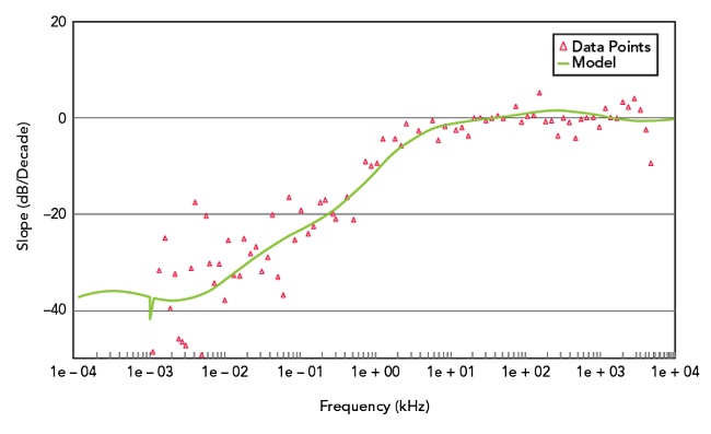
Figure 6 Slope of 50 MHz CMOS OCXO phase noise characteristic¹³ and model.

The phase noise analysis tool creates a numerical model from discrete phase noise data. The tool includes an adaptive algorithm to identify spurious deterministic components in the phase noise data. It also creates a physics-based numerical model for the random noise component of the phase noise. The tool includes a means for integrating the phase noise model and input phase noise data using a brick-wall and first-order bandpass filter with a numerical integration algorithm developed to provide accurate integration of input phase noise data with as little as a single frequency/phase noise data point per decade of frequency.

Detailed program operation and case studies of measured and simulated sets of phase noise data to validate the accuracy of the model and its features are documented by the author.^14,15 The phase noise tool is implemented in Octave¹⁶ and C and is freely available.

References

1. A. Kuo, T. Farahmand, N. Ou, S. Tabatabaei and A. Ivanov, “Jitter Models and Measurement Methods for High-Speed Serial Interconnects,” International Conference on Test, October 2004, pp. 1295–1302.
2. Phase Noise and Jitter Calculator, Abracon, Web: https://abracon.com/phase-noise-and-jitter-calculator#.
3. Phase Noise to Jitter Calculator, Marki Microwave, Web: https://rf-tools.com/jitter/.
4. Phase Noise Conversion to Phase Jitter, Excel Workbook, SiTime Corporation, Web: https://www.sitime.com/sites/default/files/uploads/SiTime-Phase-Noise-Spreadsheet-Calculator.xls.
5. Confirming Spurious, E5001A SSA-J Precision Clock Jitter Analysis, Keysight, Web: https://rfmw.em.keysight.com/wireless/helpfiles/e5052b/index.htm#data_analysis_and_data_output/data_analysis/confirming_spurious.htm.
6. F. N. Hooge, “1/f Noise Sources,” IEEE Transactions on Electron Devices, Vol. 41, No. 11, November 1994, pp. 1926–1935.
7. T. E. Parker, “Characteristics and Sources of Phase Noise in Stable Oscillators,” 41st Annual Symposium on Frequency Control, May 1987, pp. 99-110.
8. M. S. Keshner, “1/f Noise,” Proceedings of the IEEE, Vol. 70, No. 3, March 1982, pp. 212–218.
9. E. S. Ferre-Pikal and F. Walls, Frequency Standards, Characterization, Wiley Encyclopedia of Electrical and Electronics Engineering, p. 770, Web: https://tsapps.nist.gov/publication/get_pdf.cfm?pub_id=105599.
10. D. B. Leeson, “A Simple Model of Feedback Oscillator Noise Spectrum,” Proceedings of the IEEE, Vol. 54, No. 2, February 1966, pp. 329–330.
11. D. B. Leeson, “Oscillator Phase Noise: A 50-Year Review,” IEEE Transactions on Ultrasonics, Ferroelectrics and Frequency Control, Vol. 63, No. 8, August 2016, pp. 1208–1225.
12. Phase Noise Measurement in Crystal Oscillators, Application Note QTAN‐107, Q-TECH Corporation, p. 4, Web: https://q-tech.com/wp-content/uploads/QTAN107-Phase-Noise.pdf.
13. Low Phase Noise, Space Level OCXO, Datasheet, Q-TECH Corporation, Web: https://q-tech.com/wp-content/uploads/QPDS-0008-QT4100-OCXO.pdf.
14. S. M. Logan, "Octave Based Phase Noise Analysis Tool," v1.2, February 2, 2023, Web: https://www.dropbox.com/s/fo6ovy43s9usxju/phase_noise_analysis_tool_020223v1p2.pdf?dl=0.
15. S. M. Logan, "Background, Description, and Case Studies for Phase Noise Analysis Tool pnoisev2 v2.2," April 29,2024, v1.0, URL: https://1drv.ms/b/s!AnM-GsAEZPoSsTfdzwzZwtN3_q1e?e=aq9X6F.
16. J. W. Eaton, D. Bateman, S. Hauberg and R. Wehbring, "GNU Octave Version 7.3.0 Manual: A High-Level Interactive Language for Numerical Computations," Web: https://www.gnu.org/software/octave/doc/v7.3.0/.