The approach used to generate Figure 2 followed a typical post-processing application of PCA, where the data set was processed as a whole after all measurements were complete. The implementation of PCA in a real-time environment, however, requires a slightly different approach. Figure 3 shows a flowchart of a real-time PCA algorithm.
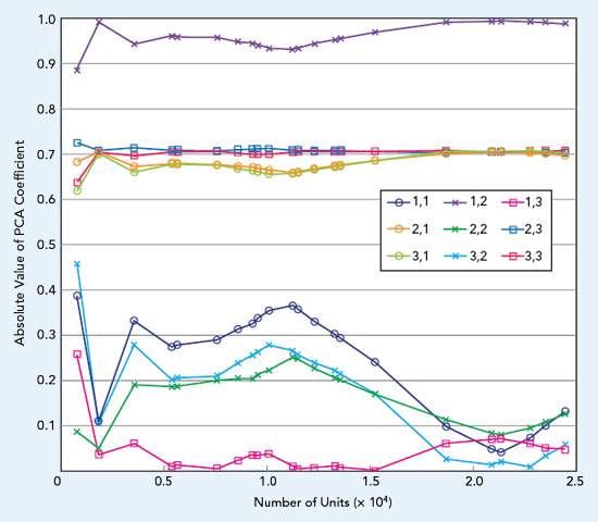
The first step in the algorithm is to load the PCA coefficient matrix, Y, into the automated test equipment. To determine Y, we discounted a real-time method, since the calculations to generate this matrix are computationally expensive and not conducive to a production environment. Instead, we used a series of previous measurements of the same LNA type to determine Y using the method described by Equations 1 through 3. For example, consider the CMD185P3 LNA with n = 3 (IDD, gain and noise figure). Figure 4 shows the absolute value of each element in the Y-matrix as a function of the number of units in the calculation. Note that as the number of units increases, the coefficients begin to converge, especially the larger ones. While convergence is not universal, this result suggests that using a larger set of training data is preferred over a smaller set.
The second step in the algorithm is to run the production test until a fixed number of units pass the electrical specifications. Recall that Equation 1 requires statistics for each of the n parameters to perform the normalization, so an initial set of measurements is needed to generate these statistics. Note that the median instead of the mean is used in the normalization equation, as this approach led to slightly better identification of outliers. The size of the initial window is variable, so after some experimentation, we chose 50 units as a compromise between having enough data to generate the statistics and not requiring an excessive amount of test time, since these units are returned to the untested population prior to outlier detection using PCA.
The third step is to restart the production test and apply PCA to each measurement. The kth unit is measured, and if any values in the vector Sk fail their respective electrical specifications, the unit is placed in the “fail” bin without further analysis. If the unit passes electrical specifications, its performance is combined with the previous 49 passing units to determine a new median and standard deviation. By using a rolling window and computing a new median and standard deviation with each unit, the algorithm accounts for a slight drift with time in the measured data. The Sk vector is then normalized to generate Xk, which is multiplied by the Y-matrix to determine the Tk vector score. If any of the values in Tk are outside the PCA cutoff parameter, this unit is considered an outlier and is placed in the fail bin. Otherwise, the unit is placed in the pass bin, and the test moves to the next unit in the sequence. The algorithm is repeated until all units in the lot have been tested.

Figure 4 Absolute value of the PCA coefficients for the CMD185P3 LNA. The legend shows the row, column entry of the Y-matrix.

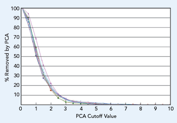
Figure 5 Simulated percentage of LNAs removed by PCA vs. the cutoff value, using measured data from 16 lots of the CMD132P3 LNA.

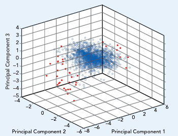
Figure 6 Real-time Tk vector scores for each CMD185P3 LNA tested in production, with cutoff parameter scores > 4 shown in red.
A major variable is the PCA cutoff parameter. A low cutoff removes too many parts, a high cutoff removes too few. To determine an appropriate value, several simulations were run using the algorithm of Figure 3, where the PCA cutoff parameter was varied to determine the number of outliers removed. Figure 5 shows the results of one set of simulations involving 17 lots of data for the CMD132P3 LNA, where each lot contained 1000 to 5000 units. The plot shows the percentage of units removed as outliers versus the cutoff value, which was varied from 0 to 10.
Although not shown, very similar results were generated from simulations of other LNAs. Based on these simulations, we chose to implement a cutoff score of 4 in the real-time application of the algorithm, which should categorize approximately 1% to 3.5% of the units as outliers and place them in the fail bin.
ALGORITHM ON THE PRODUCTION FLOOR
The algorithm shown in Figure 3 was implemented during a recent production test of a lot of CMD185P3 LNAs containing 2575 units. Again, the measured parameters were gain, noise figure and IDD (n = 3), and the window size was 50 and the PCA cutoff score set at four. Figure 6 is a graph of the Tk vector scores for each unit, where the circles in blue represent a pass, while the red circles represent the units identified as outliers and sent to the fail bin. The algorithm failed 38 outliers and passed 2454 units, an outlier removal rate of 1.5%. An additional 83 units did not pass the electrical specifications and were ignored by the algorithm.
Figure 7 shows this data in a slightly different form: each of the measurements as a function of unit number using the same color scheme, i.e., blue represents a unit that passed and red an outlier that failed. The vast majority of units removed by the algorithm had higher than average noise figure, and many of those correlated with lower gain. The algorithm did not add any time to the production test.
CONCLUSION
We have described a real-time PCA algorithm deployed on the production floor to remove outliers from the testing of the CMD185P3 amplifiers. Of the LNAs meeting the electrical specifications, the algorithm identified 1.5 percent as outliers, which was consistent with the expectation, given the cutoff score of four. We are continuing to deploy this algorithm on the production floor with numerous LNAs as we work to refine the coefficient matrix, Y, and examine the cutoff score to more effectively remove outliers from the passing population. We are also working to deploy the algorithm on other MMICs, such as driver and power amplifiers, distributed amplifiers and switches.

Figure 7 Measured IDD (a), gain (b) and noise figure (c) of the CMD185P3 LNA, showing the outliers removed by the algorithm in red..
ACKNOWLEDGEMENTS
The authors acknowledge the following for their contributions to this work: Dr. Kavitha Chandra of the University of Massachusetts-Lowell, for her guidance and introduction to PCA. This work would not have been successful without her help. Sarah McKinley and Emma Fournier of Custom MMIC helped run and improve the MATLAB simulations, and Helen Leung of Custom MMIC who deployed the algorithm on the production test equipment.
References
- H. Stratigopoulos, “Machine Learning Applications in IC Testing,” 23rd IEEE European Test Symposium, 2018.
- E. Yilmaz, S. Ozev and K. Butler, “Adaptive Multidimensional Outlier Analysis for Analog and Mixed Signal Circuits,” Proceedings of the 2011 IEEE International Test Conference, 2011.
- A. Jauhri, B. McDanel and C. Connor, “Outlier Detection for Large Scale Manufacturing Process,” IEEE International Conference on Big Data: Big Data 29, 2015, pp. 2771–2774.
- H. C. M. Bossers, J. L. Hurink and G. J. M. Smit, “Online Univariate Outlier Detection in Final Test: A Robust Rolling Horizon Approach,” Proceedings of the 16th IEEE European Test Symposium, 2011, p. 201.
- P. O’Neill, “Production Multivariate Outlier Detection Using Principal Components,” Proceedings of IEEE International Test Conference, 2008.
- B. Deschamp, “Analysis of Mammalian Cell Culture Data, Ph.D. Dissertation,” University of Massachusetts-Lowell, 2018.
- A. Nahar, R. Daasch and S. Subramaniam, “Burn-In Reduction Using Principal Component Analysis,” Proceedings of the IEEE International Conference on Test, 2005.
