In developing microwave models, real-time verification of characterization data should be considered a priority to ensure its integrity. Sound models must be built upon accurate measurement data, and, as is generally the case, the ‘garbage in – garbage out’ principle applies to model extraction. Even if an instrument calibration is rigorously inspected prior to data acquisition, there are a multitude of things that can occur after calibration to seriously degrade data integrity — damaged connectors, bent probes, cable movement, improper die attachment, warped boards, temperature variation, etc. Sometimes the errors are difficult to detect and can best be identified using real-time data analysis.

Data storage is another aspect worthy of consideration, particularly when large amounts of data are involved. The development of a single, robust model that is representative of a microwave device typically requires measurements of 5 to 10 samples, often in multiple configurations and/or test fixtures. Thus, the characterization process can result in the generation of hundreds of data files. Under these circumstances, manual generation of filenames is almost certain to lead to errors, including an S-parameter data set being associated with an incorrect bias setting or configuration, for example. Further down the model extraction process, such errors will inevitably lead to a loss of engineering time and, possibly, incorrect models.

In this article, total loss calculations are shown to be good and useful indicators of measurement quality for passive microwave components. Such calculations can be performed in real-time and provide a single, visible ‘snapshot’ that is readily evaluated as, for most components, the forward and reverse loss factors should be substantially equal. A LabVIEW program has been written to automate the loss factor calculations, control multiple test instruments, and to implement an efficient data file generation and storage process.

Loss Factor Basics

The forward and reverse loss factors are calculated from passive component S-parameters as

Forward Loss Factor (FLF) =

1 – |S11|2 – |S21|2

Reverse Loss Factor (RLF) =

1 – |S22|2 – |S12|2

By these definitions, the loss factors are seen to equal the difference between a normalized input power and the power that is reflected and transmitted to the input and output ports, respectively. (Power loss can occur due to conductor, dielectric and radiation loss mechanisms.) For reciprocal devices S21 = S12, the differences between the forward and reverse loss factor occur due to differences in |S11| and |S22|. For ideal lossless components, the magnitudes of S11 and S22 are equal, but they can deviate from one another whenever loss is present.

For passive components such as capacitors, inductors and resistors (and diodes), the electrical behavior is most often symmetrical (S11 = S22); thus, the difference in the forward and reverse loss should be negligible. Significant deviations in the forward and reverse loss can be observed when a component begins to radiate, a commonly observed phenomenon, particularly for inductors. However, the main objective of this article is to illustrate how real-time monitoring of loss factor behavior becomes a useful tool for detecting measurement inconsistencies when, all things functioning properly, the component should exhibit symmetrical characteristics.

Measurement Examples

		Fig. 1 S21 of a delay line used during a TRL calibration on FR4 substrates of different thickness.

The variation of the loss factor with frequency can often be used as a measure of data integrity. For most passive devices, the loss factor tends to increase with frequency with peaks near resonant points, such as the cut-off frequency of a filter or a self-resonance of an RLC component. A trend other than this generally indicates a measurement problem that can stem from a poor calibration, poor quality test fixtures, or other defects such as those mentioned at the beginning of this article.

Differences in the variation of loss factor with frequency are shown herein by comparing data for a 5.6 pF 0603 capacitor, as measured on 5-mil-thick and 59-mil-thick FR4 substrates. The S21 data for a delay standard of a multi-line thru-reflect-line (TRL) calibration,1 performed prior to the capacitor measurements, is shown in Figure 1. The data taken on the 5-mil substrate shows a uniform, monotonic decrease as expected, while that for the 59-mil substrate is relatively noisy. In particular, the 59-mil data shows spikes at ~4 and ~8.5 GHz. The measured S-parameters for the capacitors are given in Figure 2. While there are noticeable differences between the substrates due to ground-related parasitic effects,2 the data for each has uniform variation and excellent symmetry between S11 and S22. The variation in the loss factor, however, reveals an inconsistency in the 59-mil data. While the 5-mil data shows the expected increase in loss factor (and a spike near the resonance) the data on the thicker substrate has a small spike near 4 GHz and decreases near 8.5 GHz, as shown in Figure 3.

	Fig. 2 S-parameters for a 5.6 pF 0603 capacitor on (a) a 5-mil FR4 substrate and (b) a 59-mil FR4 substrate.

In this example, the calibration data on the 59-mil substrate clearly indicated an upper frequency limit for trustworthy data, and the problem arising in the loss factor behavior could be anticipated. Less obvious sources of error, such as poor probe contact to an uneven test fixture, are also possible and can easily result in similarly bad data. The main point here is that the non-physical behavior — decreasing dissipation near 8.5 GHz — is more apparent in the loss factor than it is in the S-parameters. Identifying this upper frequency limit is important if one is attempting to obtain high precision data.

	Fig. 3 Forward (solid line) and reverse (circles) loss factor measured on a 5.6 pF 0603 capacitor.

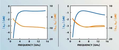
Even when the loss factor increases monotonically with frequency, asymmetry between the forward and reverse properties can be indicative of a measurement problem. Measured S-parameters for a 1.0 pF 0201 capacitor, as measured on a 5-mil substrate, are shown in Figure 4. Analyzed individually, either set of S-parameters has uniform variation and no obvious inconsistencies. However, the data on the left has nearly identical S11 and S22 characteristics, while the data on the right shows some asymmetry. A comparison between the two also indicates that S21 for the asymmetric data set is lower than the symmetric data by approximately 0.6 dB at the high end of the frequency band.

	Fig. 4 Two measurements of S-parameters for a 1.0 pF 0201 capacitor on a 5-mil-thick FR4 substrate.

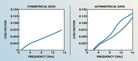
The difference between the data sets is more readily recognized by a comparison of the loss factors (see Figure 5). The symmetric S-parameters show nearly identical forward and reverse loss factors. However, the forward and reverse dissipation calculated from the asymmetric data set are different, and the loss is 60 to 70 percent higher than the symmetric results at the upper frequency limit. These two data sets were obtained from the same part and test fixture during different measurement sessions, with equal-quality instrument calibration. Thus the differences can be attributed to an inadvertent cable movement, probe placement differences, or similar post-calibration circumstances.

	Fig. 5 Forward and reverse loss factors for a 1.0 pF 0201 capacitor on a 5-mil FR4 substrate.

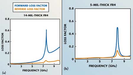
Given the preceding examples, it is worth mentioning that asymmetric S-parameters, and corresponding differences in the forward and reverse loss factor, are not necessarily incorrect. Figure 6 shows the S-parameters for a 24 nH 0603 chip inductor, as measured on 14-mil and 5-mil FR4 substrates. The data from the 14-mil substrate shows noticeable asymmetry beyond 5.5 GHz, while the 5-mil data shows a difference only near 8 GHz. These effects are due to radiation loss, which is frequently shown to be highly dependent on the substrate to which the part is mounted and on the side of the part to which the RF signal is injected. The corresponding loss factor data (see Figure 7) demonstrates that on the thicker substrate 60 percent of the incident power can be lost in one direction, while only 10 percent may be lost from the other. These radiation properties have been experimentally validated by others.3

	Fig. 6 S-parameters for a 24 nH 0603 inductor on (a) 14-mil and (b) 5-mil-thick FR4 substrates.

	Fig. 7 Loss factors calculated from S-parameters for a 24 nH 0603 inductor on (a) 14-mil and (b) 5-mil-thick FR4 substrates.

Measurement Automation

		Fig. 8 Sample screen from the LabVIEW measurement-control program.

The best time to validate experimental data is when the measurements are being made. Errors that are caught down-stream, perhaps stemming from an equipment problem that occurred after calibration, can result in a significant amount of lost engineering time. Currently, however, most software that is commercially available for microwave measurements and data extraction does not allow user-defined equations to be generated for data analysis purposes.

A LabVIEW program was written in order to implement real-time loss factor analysis, as well as an automated filename generation algorithm. A sample front-panel screen shot is shown in Figure 8 and the elements of the program are summarized in Table 1. Information-rich filenames are created by concatenating parameters such as internal job number, component description and test fixture identifiers. Additional features of the program enable GPIB-control of bias supplies and various meters to facilitate active device characterization from a central command point.

	TABLE I ELEMENTS OF THE LabVIEW PROGRAM Stage National Instruments Library VIs Description Initialize VNA AW372XXA INT open VNA.vi initialize GPIB communication with the VNA Setup channel format CH graph type.vi set up each channel in the desired display and data format Measure button while loop wait to proceed until the “measure” button is pushed Sweep frequency AW372XXA DAT frequency values.vi obtain frequency points from VNA Sample channels AW372XXA DATA get trace.vi obtain data 4 times (once for each parameter) Calculations standard “numeric” and equation functions perform desired calculations Display data XY graphs standard XY graph display Data format and saving while loop, write file wait to proceed until “save” or “reset” is pushed and save if needed

Conclusion

Loss factor calculations using measured S-parameters are simple to perform, and provide useful insight into data quality for passive, reciprocal components. Loss factor ties the port-matched transmission and reflection coefficients together, is symmetric for a physically symmetric component and should generally increase with frequency (except after a peak near resonance). Since myriad problems can arise during high frequency measurements to degrade the accuracy, tracking a parameter whose general properties are known a priori is a valuable aid when measurement precision is critical.

Acknowledgment

The authors would like to thank Carl Petersen of National Instruments (www.ni.com/labview) for his assistance with the LabVIEW program development.

References

1. R.B. Marks, “A Multi-line Method of Network Analyzer Calibration,” IEEE Transactions on Microwave Theory and Techniques, Vol. 39, No. 7, July 1991.
2. V. Cojocaru, et al., “Enhancing the Simulation Accuracy of RF Designs with Consistent Characterization and Modeling Techniques,” 59th Conference on Automatic Radio Frequency Techniques (ARFTG), Boulder, CO, March 2002.
3. E. Benabe, et al., “Substrate-dependent Air Wound Inductor Model in the DC-4 GHz Range,” 54th Conference on Automatic Radio Frequency Techniques (ARFTG), December 1999.

John A. Capwell received his BSEE degree from the University of South Florida in 1999 and is currently pursuing his MSEE degree from the same university. He is a member of the technical staff at Modelithics Inc. and works in the areas of microwave measurements, and active and passive component modeling.

Tom Weller received his BS, MS and PhD degrees in electrical engineering from the University of Michigan in 1988, 1991 and 1995, respectively. He was a member of the technical staff at Hughes Space & Communications Group from 1988 to 1990. He is currently an associate professor in the department of electrical engineering at the University of South Florida, and a member of the Wireless and Microwave (WAMI) Center. He co-founded Modelithics Inc. with Larry Dunleavy in 2001.

David P. Markell received his BSEE degree from the University of South Florida in 1998 and is currently pursuing his MSEE degree from the same university. He is currently a member of the technical staff at Modelithics Inc. His research interests include semiconductor theory, transistor and diode modeling.

Lawrence P. Dunleavy received his BSEE degree from Michigan Technological University in 1982, and his MSEE and PhD degrees from the University of Michigan in 1984 and 1988, respectively. He has worked in industry for E-Systems (1982-1983) and Hughes Aircraft Co. (1984-1990), and was a Howard Hughes Doctoral Fellow (1984-1988). In 1990, he joined the electrical engineering department at the University of South Florida, where he holds the title of professor. He is a senior member of IEEE, and is very active in both the IEEE MTT Society and the Automatic RF Techniques Group (ARFTG). He has authored or co-authored seventy technical articles. In 2001, along with Thomas Weller, he founded Modelithics Inc.