
RF Wireless Power: A to Z
For many years, the capabilities of long-range wireless power have been talked about and with increasing interest. The technology is proven and is already being used today in many industries like manufacturing, building automation and hospitality. An assortment of other, short-range wireless charging technologies are on the market, including Qi (inductive coupling) and magnetic resonance. However, the focus of this article will be on the various methodologies for RF-based wireless power for powering devices over distance.
WIRELESS POWER OVER DISTANCE
RF wireless power is a technology that enables power to be sent over distance using radio waves. A transmitter uses an antenna to generate an RF field which propagates toward a receiver’s antenna. The receiver captures a portion of the RF field and uses an RF to DC converter to produce usable DC to power electronics or recharge batteries. RF wireless power can be implemented in various ways and many design decisions impact the performance of the system. When all variables are considered, RF wireless power networks offer a way to remove wires and batteries from many of the devices we encounter every day.
Wireless power transmission using RF in the far field can be described using the Friis equation:

where PR is the received power, PT is the transmitted power, GT( θT,φT) is the angular dependent transmitter antenna gain, GR( θR,φR) is the angular dependent receiver antenna gain, λ is the wavelength, r is the distance between the transmit and receive antennas, ΓT is the transmit antenna reflection coefficient, ΓR is the receive antenna reflection coefficient, p̂T is the transmitter antenna polarization vector and p̂R is the receiver antenna polarization vector. Generally, the transmitter and receiver are assumed to be matched, have the same polarization vectors and are in the main radiation beam, which simplifies the equation to:

This equation shows the received power is inversely proportional to the distance squared, which means if the distance doubles, the received power reduces by 4x. This can be understood considering the power is spreading over the surface area of a sphere with area A=4πr2.
Another factor in RF wireless power transfer is the received power is proportional to the square of λ or inversely proportional to the square of the frequency. This means a low frequency signal will provide more received power than a higher frequency signal, assuming all other variables are the same. For example, consider an amplifier delivering 1 W of RF power to a transmitting antenna with a gain of 4, i.e., 4 W EIRP. A dipole antenna at a fixed distance at 915 MHz will receive about 7x more power than a dipole antenna at 2.4 GHz:

and about 40x more power than a dipole at 5.8 GHz:

This difference in power is because the effective area of the antenna is reducing as frequency increases. The dipole antenna, typically λ/2 long, gets shorter as frequency increases, reducing the physical capture area of the antenna.
However, the power density, S, is independent of frequency:

Equation 3 shows the radiated power spreads over the surface of a sphere independent of frequency, and the effective area of the antenna, also known as capture area, determines the amount of received power. This explains why a λ/2 dipole antenna at 5.8 GHz captures less energy than a λ/2 antenna at 915 MHz under identical conditions.
The effective area of an antenna, Ae, is directly proportional to its gain:


Figure 1 Far-field boundary where spherical waves approximate a plane wave.
Higher gain antennas can be used to increase the capture area, but high gain antennas come at the cost of directionality. Depending on the application, precise antenna directionality is not always advantageous. One way around this potential burden is using multiple antennas and RF to DC converters to increase the overall capture area. However, this solution also increases the cost of the receiver because of the additional hardware. This shows why it is important to outline performance and project expectations prior to designing the system.
The Friis equation is only valid in the far field, so determining the boundary between the near and far field is important. One common method is to determine where the parallel ray approximation begins to break down, i.e., where the wave exiting the transmit antenna can be approximated as a plane wave impinging on the receiving antenna. A plane wave means the receiving antenna sees a constant amplitude and phase across its aperture (see Figure 1). Typically, a phase error of π/8 or 22.5 degrees across the receiving aperture is considered an acceptable approximation for a plane wave, which yields the common boundary between the near and far fields given by:

where D is the maximum dimension of the transmitting or receiving antenna or array, r is the distance between the transmitting and receiving antennas and λ is the wavelength.
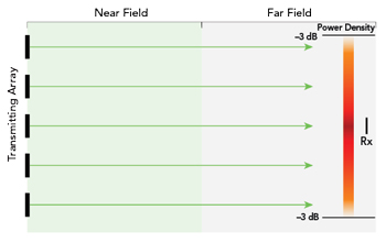
Figure 2 Far-field focusing.

Figure 3 Near-field focusing.
BEAM FOCUSING, POWER DENSITY SPOT SIZE
In some applications, it is advantageous to focus the RF field onto a receiving antenna to maximize power throughput. This can be done several ways, usually through far-field focusing (see Figure 2) or near-field focusing (see Figure 3) of the RF power to increase power density. The far-field technique is usually referred to as beamforming or beam steering and is accomplished with a high gain antenna or by using an antenna array focused at an infinite distance to produce a directional beam. The direction of the beam is controlled by either mechanically or electronically directing the signal toward the receiving antenna. With near-field focusing, an antenna array typically focuses each antenna element to a finite point in the near field to produce a hot spot of RF power density, with the subsequent fields for each antenna diverging in the far field beyond the hot spot.
With far-field beamforming, it is important to understand the limitations of “focusing” the RF energy. The size of the beam and the focus area will always be bigger than the physical dimensions of the transmitting antenna. Focusing the rays from each antenna element at an infinite point in the far field means the rays are parallel, as seen in Figure 2. However, the ray from each antenna element will spread over distance per the far-field beamwidth specification in the datasheets of commercially available antennas. A narrow beam’s aperture begins as the minimum size of the antenna and spreads as it travels. Therefore, if the transmitting array is 1 m2, the beam will never be smaller than 1 m2, which is important when sending RF power to a receiving antenna smaller than the transmitting antenna. While beamforming does focus more RF power to a receiving antenna, a large portion of the steered beam may be outside the desired capture area.
With near-field focusing, the rays from each antenna converge on a point in the near field to form a localized spot of high RF power density, as shown in Figure 3. The -3 dB (i.e., half power) size of the spot can be as small as slightly less than λ/2. Depending on the dimensions of the receiving antenna, the spot can be comparably sized to the receiving antenna. If the two are similarly sized, more efficient coupling can be achieved between the transmitter and receiver. However, since this solution is more closely coupled, the system should be simulated and designed as a whole, meaning both the transmit and receive antennas. Due to the proximity of the antennas, their impedances can change, and the amplitude and phase of the field across the receiving antenna aperture are likely not uniform. While far-field antennas are designed with consistent amplitude and phase across their capture areas (i.e., assuming plane waves), typical antenna design practices may not apply for near-field operation, so system simulation is vital for optimizing the performance of a near-field wireless power solution.
Both far-field and near-field focusing can provide higher throughput of RF wireless power. However, this is achieved incurring complexity, which often increases cost. A beam focusing solution may contain mechanical or electronic steering, like a motor or amplitude and phase adjusting circuitry. This increased cost makes the wireless benefits difficult to justify. As a transmitter with a single antenna and amplifier will be much smaller and significantly less expensive than a beam focusing solution, this approach is more viable for high volume applications.
BUILDING MATERIALS
As RF wireless power propagates through various dielectric materials, antennas can be embedded inside a product because line of sight between the transmitter and receiver is not necessary. This also means wirelessly powered sensors can be permanently embedded into building materials and placed behind walls. Typical indoor building materials like drywall are “RF friendly,” as we know from the proliferation of Wi-Fi.
Considering the impact of walls on RF wireless power transfer, several properties impact power delivery. All dielectric materials have a dielectric constant (i.e., relative permittivity) and a loss tangent. Typically, a dielectric material is characterized by its loss or how it attenuates the RF signal propagating through it. This loss is related to the loss tangent of the material, which can be quite low for materials like drywall and will be greater for masonry like brick and concrete. Since the dielectric constant of the material is greater than the dielectric constant of the air inside the room, the difference creates an interface between the mediums that causes a refraction and reflection of the wave off the surface of the material.
The amount of reflected power and the angle of reflection depend on the polarization of the wave with respect to the plane of incidence and are described by the Fresnel equations. For simplicity, the following equations assume a lossless, non-magnetic dielectric:


Figure 4 Calculated transmitted and reflected power of an incident wave on a lossless, non-magnetic drywall boundary (εr = 2.19).
where RS is the power reflection coefficient for the perpendicular polarization, RP is the power reflection coefficient for the parallel polarization, θi is the angle of the incident wave, θt is the angle of the refracted wave and ε1 and ε2 are the dielectric constants of the two media.
Plotting these equations (see Figure 4) shows the reflected and transmitted power at the interface. Incident angles less than 60 degrees enable 80 percent or more of the RF wireless power to transmit into the wall. Interestingly, with parallel polarization, 100 percent of the RF wireless power transmits into the wall at Brewster’s angle.
Because a sheet of drywall is not lossless and creates two interfaces—room into the drywall and drywall to the air behind it—a simulation using Ansys HFSS helps visualize how drywall affects propagation. The scenario comprised 12.8 mm thick drywall with εr = 2.19, tan δ = 0.0111 and a 915 MHz transmitting dipole antenna located 0.5 m from the wall. The magnitude of the electric field (E-field) was plotted for a 4 × 2 m plane of incidence with perpendicular polarization (see Figure 5a). For comparison, the simulation was repeated with the wall removed (see Figure 5b). The figures show top-down views of the plane of incidence, i.e., the dipole and wall project into and out of the page.

Figure 5 Top view of the E-field magnitude with (a) and without (b) drywall boundary.
The simulation without the wall (Figure 5b) shows smooth, even E-field rings. In Figure 5a, the portions of the rings at angles of incidence near zero (i.e., directly down from the dipole) show results similar to the no-wall example because of little reflection off the drywall, i.e., due to the small angle of incidence. At steeper angles—at the far right and left of the dipole—the reflected E-field is higher, causing more distortion of the rings. The reflected waves are constructively and destructively interfering with the main E-field from the dipole. Examining both images, the two simulations share a similar E-field due to the relatively low dielectric constant of the drywall, with minimal RF reflection. The simulation confirms RF wireless power can be implemented without line of sight as long as the system is designed for it. Even with a wall separating the transmit and receive antennas, power delivery is possible, relatively unaffected by the barrier.
CONCLUSION
RF wireless power can be implemented in vastly different ways. Due to the complexity of each environment, various system parameters can be adjusted to meet the demands of an individual application. In general, lower frequency signals have greater RF power throughput. The size of the receiving product typically sets the maximum antenna size, which dictates the minimum frequency for power delivery. While it is possible to use electrically small antennas, these have a narrow bandwidth which makes them impractical for mass production from shifts in resonant frequency caused by manufacturing tolerances.
Focusing the RF in the near field or far field offer additional ways to increase throughput. However, including multiple antennas in an array with supporting electronics multiplies the cost of a deployment, so a transmitter with a single antenna and amplifier may be more advantageous for high volume applications. The presence of standard indoor building materials has minimal impact on the RF field, so multi-room RF wireless power systems are possible.
Given the design options, RF wireless power systems can be engineered to meet the different needs of many applications in many market verticals. RF wireless power is not a technology of the future; it is a technology being deployed today, with rapid expansion and mass adoption on the near-term horizon.