Online Spotlight: Legacy Standards and Test Methods Limit the Use of Modern Spectrum & Signal Analyzers

Spectrum analyzers have quickly evolved and made huge technological leaps from the initial instruments created in the 1960s, especially with the discovery of the fast Fourier transform (FFT); however, since most signals today are not continuous, but are modulated, some legacy measurement methods are simply not good enough and can lead to incorrect results.

Examination of a signal in the frequency domain is one of the most frequent tasks in radio communications, and such a task would be unimaginable without modern spectrum analyzers. Those instruments can analyze a wide range of frequencies and are irreplaceable in practically all applications of wireless and wired communications. With technological advancements, more is expected of spectrum analyzers, including the analysis of average noise levels, wider dynamic range and increased testing speed.

THE ORIGINAL SPECTRUM ANALYZER

Since the original spectrum analyzers were developed, the architecture has been based on an analog heterodyne receiver principle. The area circled in red in Figure 1 comprises real analog components. These components are responsible for rectifying the down-converted input RF signal to a video signal or voltage. The signal is further processed to determine how the result is displayed on the screen. A CRT type display in the early days allowed the user to view the measurements.

Figure 1 Original spectrum analyzer block diagram.

Figure 2 Modulated RF waveform.

Figure 3 Rectified waveform.

The spectrum analyzer is only interested in the amplitude of signals in the frequency domain and in the early years, as now, people were mostly interested in the power of the spectral components. The envelope detector circuit converts the signal, either a continuous wave (CW) or modulated RF waveform (see Figure 2) and rectifies it, resulting in a video (envelope) voltage (see Figure 3).

Of course, the combination of a log amp and envelope detector is logarithmic in nature and, for that reason, early measurements with spectrum analyzers that dealt with power were always treated as logarithmic quantities. It is obvious that the unit of dBm is a logarithmic quantity, but the voltage data from the very first conversion starts as logarithmic; then, the data reduction that happens further in processing can cause some interesting effects.

RMS POWER AS THE TRUE POWER MEASUREMENT

In the past, power measurements were made using logarithmic detection. The peak detector was “calibrated” to show the correct level for CW tones and, in the early days, the measurement of CW signals was most likely sufficient. Using trace averaging reduces the level of noise shown on the trace. Because carrier power measurement - not noise power measurement - was the focus, engineers rarely converted values to linear quantities (e.g., watts) prior to performing averaging. Instead, the instrument performed trace averaging by simply averaging the dBm values.

Using trace values represented as x in the equations below, the usual method employed in early analyzers was simply to sum up the logarithmic values and calculate the average:

The correct way to do it is to convert the logarithmic values to linear values, calculate their linear average, then re-convert them to logarithmic values at the end:

Today, signals are not just CW but often incorporate some sort of modulation, so the method of measuring those signals correctly needs to change to measure the correct power level for both the carrier itself and its adjacent noise quantities. The notable standards setting organizations, such as the NPL (National Physical Laboratory) in the U.K., the PTB (Physikalisch-Technische Bundesanstalt) in Germany and NIST (National Institute of Standards and Technology) in the U.S., typically measure root mean square (RMS) power. From Ohm’s law, P = V²/R is the RMS power produced. This is accepted worldwide as the standard measure of power; it is fully defined and understood.

COMPARISON OF LOGARITHMIC AVERAGING VS. RMS TRUE POWER MEASUREMENTS

In early spectrum analyzers, the available detectors were typically peak, sample or minimumpeak, and these do not distinguish between linear or logarithmic values, since a peak is a peak (see Figure 4). There are three traces, each measuring a CW (no modulation) signal with a marker for each trace. In this case, all three markers measure the same power level of -0.3 dBm.

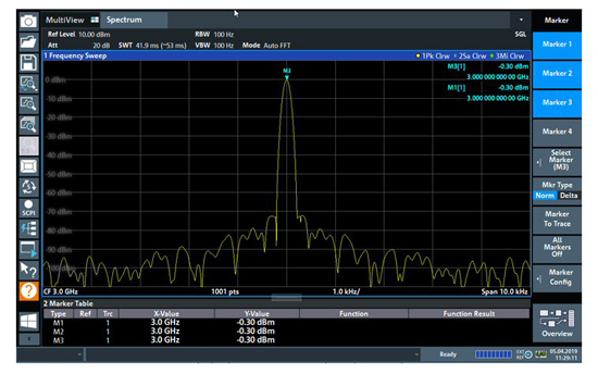
Figure 4 Display of power on an early spectrum analyzer.

This is fine for continuous waveforms, but what about modulated waveforms? Today, most signals are not CW but are modulated, and the user would benefit from using trace averaging to provide a smooth response with a high level of measurement repeatability (see Figure 5). Many signals designed to have modulation appear like Gaussian noise, so this example is highly relevant.

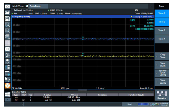
Figure 5 Modern spectrum analyzer display of a modulated RF waveform.

Here, the typical detector used in legacy spectrum analysis is the sample detector, which always picks the Nth sample out of M samples taken within a timeframe T. If trace averaging is performed on this logarithmic data (trace 1) and compared to a true RMS measurement (trace 2), the result is 2.5 dB lower than the RMS power. This could cause serious problems for the user if wrong measurement settings are applied, or trace averaging is used with legacy trace modes or detectors that are logarithmic in nature.

WHAT IS LIMITING ACCURACY AND SPEED, EARLIER STANDARDS OR TEST DOCUMENTS?

During my career at Rohde & Schwarz, I have seen many tests from customers that were written using legacy equipment, though they were meant to be implemented using modern equipment. While it is entirely possibly to perform measurements as originally intended, this leads to two fundamental problems:

• The high risk of users doing manual measurements (e.g., those that are not led by test documents or specifications) with different results in linear and logarithmic calculations due to trace averaging, resulting in measurement errors.
• Users not using more accurate, automatic linear measurements with significantly improved speed and repeatability.

HOW DO MODERN INSTRUMENTS SOLVE THIS PROBLEM?

In a modern instrument, everything beyond the IF filter is digital (see Figure 6). Even the resolution bandwidth filter (RBW) is digital. Because of this, it is much easier to include different types of detectors with true linear power characteristics. Digital signal processing now handles many things, from the sharpness and fast settling time of filters to frequency response correction. Modern instruments also come with RMS detectors standard. This allows linear trace averaging if required, and there are other interesting effects of the RMS detector depending on the type of signal analyzed.

Figure 6 Modern spectrum analyzer block diagram.

Modulated Signals

As previously mentioned, the RMS detector yields a true power measurement. The sweep time, span, RBW and sweep points define the amount of averaging within a trace. Assuming the span, RBW and sweep points are fixed, one would typically increase the sweep time rather than averaging traces to get a more averaging effect. If an FFT mode is available, more samples can be captured for the same sweep time, which results in a higher amount of averaging and smoother traces. This is typically the best choice for averaging and is great for use with modulated signals.

Continuous Waveform Signals

Close attention must be paid to the span/RBW ratio and the number of sweep points. The RMS detector does not only average over time but also over frequency, so it is required to have at least one sweep point per RBW. Using a single point per RBW can lead to measurement errors and the signal power appearing lower than actual. A useful rule of thumb is “sweep points >5x span/RBW” to provide a correct power level.

Figure 7a Signal source measured incorrectly with 1001 sweep points.

For example, Figure 7a uses an RMS detector with a CW signal over a span of 500 kHz and an RBW of 50 Hz. The output from the signal source connected to the spectrum analyzer is 0 dBm. In this case, the 5x span/RBW = 50,000, but the number of sweep points is set to 1001, and the result is a level displayed that is approximately 10 dB too low. If the number of sweep points is set to 50,001, in line with the requirements calculation, then the correct result of 0 dBm is obtained (see Figure 7b).

Figure 7b Signal source measured correctly with 50,001 sweep points.

Speed       

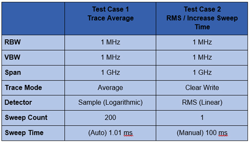
The method of using an RMS detector with increased sweep time instead of utilizing trace averaging also produces significantly faster measurements, considering results with an equivalent standard deviation. For example, consider the power measurement of a modulated, noise-like signal with a repeatability of around 0.1 dB, using the settings in Table 1.

TABLE 1

To illustrate the statistical speed improvement, a test script can measure both the time taken to retrieve a measurement result and the result itself. Over many measurements, the standard deviation of the results is calculated. On a modern signal and spectrum analyzer, the results are summarized in Table 2. The standard deviation of measured amplitude is less than 0.1 dB (see Figure 8); and, more importantly, the time taken to do the test is greater than 5 times faster using the modern RMS detector method (see Figure 9). This is true even when the sweep time of test case 1 is just 0.01 that of test case 2.

TABLE 2

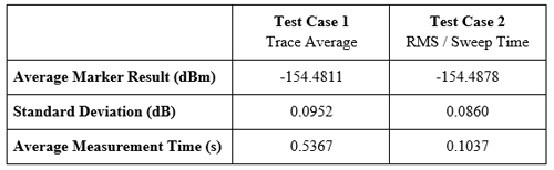
Figure 8 Comparison of measured amplitude for the trace average versus the RMS measurement method.

Figure 9 Comparison of measurement time for the trace average versus the RMS measurement method.

Running a similar set of tests with a varying sweep time, together with recording the time per measurement and the associated deviation in results, shows the improvement in test time (see Figure 10). Allowing the deviation in results to increase from 0.1 to 0.2 dB yields a further factor of 4x greater speed improvement, indicated by the red crosses on Figure 10.

Modern signal and spectrum analyzers are quite different instruments compared to those that existed 20 or so years ago. They incorporate a variety of measurement features that align with the accepted norms needed for industry today, while allowing measurements to be made using legacy methods. This can save significant time for engineers and increase measurement accuracy by using the newer incorporated features - only if engineers adopt new measurement methods versus those written in test or standards documentation from the last decades.

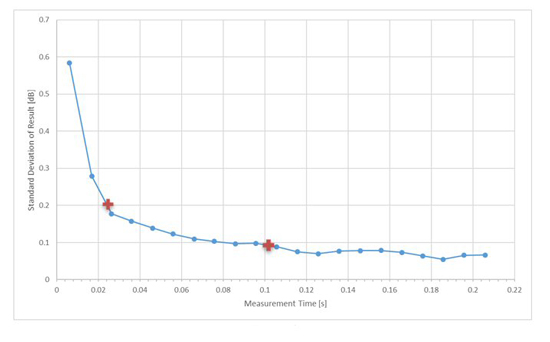
Figure 10 Standard deviation of measurement results as a function of measurement time for the RMS measurement method.