
Spatial Multiplexing for 5G Wireless Communications
Increasing demand for higher data rates and channel capacity is driving the need to use the RF spectrum more efficiently. As a result, 5G wireless systems will use mmWave frequency bands to take advantage of the increased bandwidth. The higher operating frequencies enable large-scale antenna arrays, which can be used to mitigate severe propagation loss in the mmWave band. Large arrays can also be used to implement a MIMO system in which unique signals can be transmitted from different antenna elements in the array. MIMO systems enable spatial multiplexing techniques that can be used to improve data throughput.
The core idea of spatial multiplexing is to create multiple subchannels in scatterer-rich environments so that multiple data streams can be transmitted and recovered independently. This is achieved by applying a set of precoding and combining weights derived from the channel matrix. This concept is discussed first with an all-digital solution based on precoding in a MIMO-OFDM system that uses a spatial channel model. This channel model incorporates array pattern information to improve model fidelity.
Because 5G systems require large antenna arrays, applying digital weights on each antenna element is not always practical due to cost and space limitations. Hybrid beamforming techniques can be applied in a mixed RF and digital beamforming system to alleviate these restrictions. In a hybrid beamforming system, both the precoding weights and the combining weights are combinations of baseband digital weights and RF band analog weights. On the transmit side, the baseband digital weights modulate the incoming data streams to form input signals at each RF chain, and the analog weights then translate the signal at each RF chain to the signal radiated at each antenna element. The process is reversed on the receive side. This article includes an example with hybrid weights and compares the achieved spectral efficiency with the all-digital case.
SPATIAL MULTIPLEXING
The idea behind spatial multiplexing is that a MIMO system in a multipath channel with a rich scatterer environment can send multiple data streams simultaneously across the channel. For example, the channel matrix of a 4 × 4 MIMO channel becomes full rank because of the scatterers. This means that it is possible to send as many as four data streams at once. The goal of spatial multiplexing is less about increasing the signal-to-noise ratio (SNR) and more about increasing the information throughput.
The idea of spatial multiplexing is to separate the channel matrix into multiple modes so that the data stream sent from different elements in the transmit array can be independently recovered from the received signal. To achieve this, the data stream is precoded before the transmission and then combined after the reception. In the MATLAB models that follow, the precoding and combining weights can be computed from the channel matrix by:
[wp, wc] = diagbfweights(mimompchan);
The information received by each receive array element is simply a scaled version of the transmit array element, which results in multiple orthogonal subchannels within the original channel. The first subchannel corresponds to the dominant transmit and receive directions, so there is no loss in the diversity gain. In addition, it is possible to use other subchannels to carry information, as shown by the bit error rate (BER) curves in Figure 1, including the first two subchannels. The gain of the second data stream is not as high as the first stream, since it uses a less dominant subchannel. Still, the overall information throughput is improved. This concept will be applied to a MIMO-OFDM system.

Figure 1 BER of MIMO multipath streams compared to a single line-of-sight link.
MIMO-OFDM SYSTEMS
MIMO-OFDM systems are common in wireless systems due to their robustness with frequency-selective channels and high data rates. With antenna arrays that implement spatial multiplexing, efficient techniques to realize the transmissions are necessary. As an example, consider an asymmetric MIMO-OFDM single-user system in which the maximum number of antenna elements on the transmit and receive ends are 1024 and 32, respectively, and up to 16 independent data streams. For clarity, a single link (one base station communicating with one mobile user) is modeled, but this structure could be extended for more complex configurations.

Figure 2 Channel sounding (a) and data transmission/reception (b) flow.
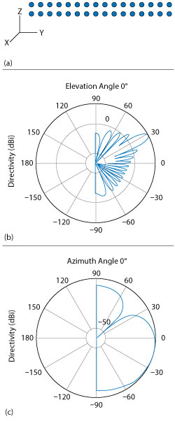
Figure 3 Transmitter array geometry (a) with azimuth (b) and elevation (c) beam patterns.
The link between the transmitter and receiver relies on channel sounding to generate the channel information needed for transmit beamforming. For a spatially multiplexed system, the availability of channel information at the transmitter allows for precoding to be applied to maximize the signal energy in the direction and channel of interest. Assuming a slowly varying channel, this process is facilitated by first sounding the channel with a reference transmission. The receiver then estimates the channel and feeds this information back to the transmitter, as shown in Figure 2. In this system, a preamble signal is first sent over all transmitting elements. It is subsequently processed at the receiver after accounting for the channel effects. The receiver performs pre-amplification, OFDM demodulation, frequency domain channel estimation and calculation of the feedback weights based on channel diagonalization using singular value decomposition per data subcarrier. The specific system configuration is as follows:
| % Single-user system with multiple streams | |
| prm.numSTS = 16; | % Number of independent data streams, 4/8/16/32/64 |
| prm.numTx = 32; | % Number of transmit antennas |
| prm.numRx = 16; | % Number of receive antennas |
| prm.bitsPerSubCarrier = 6; | % 2: QPSK, 4: 16-QAM, 6: 64-QAM, 8: 256-QAM |
| prm.numDataSymbols = 10; | % Number of OFDM data symbols |
A rectangular array at the transmitter is used, based on the desired number of data streams and transmit antennas. Figure 3 shows the array geometry of the transmitter and the beam patterns in azimuth and elevation. For simplicity, assume the steering angle is known with respect to the mobile location. In actual systems, the steering angle would be obtained from an angle-of-arrival estimation at the receiver, as a part of the channel sounding or initial beam tracking procedures.
Multiple options exist for modeling spatial MIMO channels, typically selected based on the level of fidelity that is needed for the analysis. For example, 5G channel models and the WINNER II channel models are spatially defined MIMO channels where the array geometry and location information can be specified. For this discussion, consider scattering-based channels with a single-bounce path through 100 scatterers placed randomly within a circle between the transmitter and receiver. The channel model allows path loss modeling and both line-of-sight (LOS) and non-LOS propagation conditions. For this analysis, a non-LOS propagation and isotropic antenna element pattern with linear geometry are configured. The same channel is used for both sounding and data transmission. The data transmission has a longer duration controlled by the number of data symbols.

Figure 4 Receiver array geometry (a) with azimuth beam pattern (b).

Figure 5 Constellation diagram for the MIMO OFDM system.
The receive antenna array, shown in Figure 4, passes the propagated signal to the receiver to recover the original information embedded in the signal. Similar to the transmitter, the receiver used in a MIMO-OFDM system contains many stages, including OFDM demodulator, MIMO equalizer, QAM demodulator and channel decoder. For this MIMO system, the displayed receive constellation of the equalized symbols offers a qualitative assessment of the reception. The actual BER offers the quantitative figure by comparing the actual transmitted bits with the received decoded bits (see Figure 5).
Parameters can be modified to vary the number of data streams, transmit/receive antenna elements, base station or array locations and geometry, channel models and their configurations to study the parameters’ individual or combined effects on the system. This framework can be used for further analysis but, so far, all of the precoding and combining were based on an all-digital system. As the antenna array size increases, an all-digital system may not be feasible, which leads to the use of hybrid beamforming.
HYBRID BEAMFORMING
In a hybrid beamforming system, both the precoding weights and the combining weights are combinations of baseband digital weights and RF band analog weights. This type of architecture is shown in Figure 6.

Figure 6 Hybrid beamforming architecture.
For this discussion, assume a set of larger arrays: The transmitter consists of a 64-element square array with four RF chains, and the receiver is based on a 16-element square array with four RF chains. Each antenna is connected to all RF chains, which means that each antenna is connected to four phase shifters. This type of array can be modeled by partitioning the array aperture into four completely connected subarrays. To maximize the spectral efficiency in the system, each RF chain can be used to send an independent data stream. In this case, the system supports up to four streams.
A scattering environment with six scattering clusters randomly distributed in space is used to define the channel. Within each cluster, there are eight closely located scatterers, for a total of 48 scatterers. The path gain for each scatterer is obtained from a complex circular symmetric Gaussian distribution.
As described earlier, in a spatial multiplexing system with all-digital beamforming, the signal is modulated by a set of precoding weights, propagated through the channel and recovered by a set of combining weights. Mathematically, this process can be described by Y = (X*F*H+N)*W where
- Ns is the number of data streams.
- Nt is the number of transmit elements.
- Nr is the number of receive elements.
- Nrf is the number of RF channels.
- X is an Ns-column matrix whose columns are data streams.
- F is an Ns × Nt matrix representing the precoding weights.
- H is the channel representation.
- W is an Nr × Ns matrix representing the combining weights.
- N is an Nr-column matrix whose columns are the receiver noise at each element.
- Y is an Ns-column matrix whose columns are recovered data streams.
Since the goal of the system is to achieve better spectral efficiency, obtaining the precoding and combining weights can be considered an optimization problem in which the optimal precoding and combining weights make the product of F*H*W a diagonal matrix, so each data stream can be recovered independently.

Figure 7 Transmit patterns for all-digital (a) and hybrid (b) cases.
In a hybrid beamforming system, the signal flow is similar. Both the precoding weights and the combining weights are combinations of baseband digital weights and RF band analog weights. The baseband digital weights convert the incoming data streams to input signals at each RF chain, and the analog weights then convert the signal at each RF chain to the signal radiated or collected at each antenna element. Note that the analog weights can only contain phase shifts. Mathematically, it can be written as F = Fbb*Frf and W = Wbb*Wrf, where
- Fbb is an Ns × NtRF matrix.
- Frf is an NtRF × Nt matrix.
- Wbb is an NrRF × Ns matrix.
- Wrf is an Nr × NrRF matrix.
Since both Frf and Wrf can only be used to modify the signal phase, there are extra constraints on the optimization process to identify the optimal precoding and combining weights. Ideally, the resulting combination of Fbb*Frf and Wrf*Wbb are close approximations of F and W that are obtained without those constraints. Unfortunately, optimizing all four matrix variables simultaneously is quite difficult. Many algorithms exist that arrive at suboptimal weights with a reasonable computational load. This example uses an approach that decouples the optimizations for the precoding and combining weights. It first uses the orthogonal matching pursuit algorithm to derive the precoding weights. The hybrid weights can be computed as
[Fbb, Frf] = helperHybridPrecodingWeights(H, NtRF, Ns, At);
Once the precoding weights are computed, the result is used to obtain the corresponding combining weights. Assuming the channel is known, the unconstrained optimal precoding weights can be obtained by diagonalizing the channel matrix and extracting the first NtRF dominating modes.
The transmit beam pattern for both cases is shown in Figure 7. The response patterns show that even in a multipath environment, the number of dominant directions is limited. The beam pattern using the hybrid weights is similar to the beam pattern obtained using the optimal weights, especially for the dominant beams. This result means that the data streams can be successfully transmitted through those beams using hybrid weights.

Figure 8 Spectral efficiency of all-digital and hybrid systems.
One of the system-level performance metrics of a 5G system is the spectral efficiency. Figure 8 compares the spectral efficiency achieved using the optimal weights with the proposed hybrid beamforming weights. The simulation assumes one or two data streams. The transmit antenna array is assumed to be at a base station, with a focused beam coverage of 60 degrees in azimuth and 20 degrees in elevation. The signal can arrive at the receive array from any direction. The resulting spectral efficiency curve is obtained from 50 Monte Carlo trials for each SNR. Figure 8 shows that the spectral efficiency improves significantly by increasing the number of data streams. In addition, hybrid beamforming can perform close to what optimal weights can offer and uses less hardware.
SUMMARY
MIMO systems enable spatial multiplexing techniques that can be used to improve data throughput. This improvement is achieved by applying a set of precoding and combining weights derived from the channel matrix. Because 5G systems require large antenna arrays, applying digital weights on each antenna element is not always practical. Hybrid beamforming can be applied in a mixed RF and digital beamforming system to lower system costs. System modeling techniques can be used to explore system tradeoffs before any hardware is built, which can prevent costly errors and project delays.